An implementation of the finite differences method for the two-dimensional rectangular cooling fin problem

Published Online August 2019 in MECS DOI: 10.5815/ijitcs.2019.08.01

The study of the transport equation, also known as advection-diffusion-reaction equation remains an active field of research since such an equation plays a fundamental role in a wide variety of modeling problems. Some of them are related to aerodynamics, meteorology, oceanography, hydrology, and chemical engineering [1]. In general terms, the transport equation describes how the concentration of one or more elements (pollutants, heat, etc.) which are distributed in a medium, change under the influence of three physical factors: diffusion, convection, and reaction. Convection refers to the movement of an element within a medium. Diffusion is the movement of the element from an area of high concentration to an area of low concentration, resulting in the uniform distribution of the element. Reaction is the interaction process that results in the involved elements be generated or consumed.

Formally, the two-dimensional version of the transport equation is a partial differential equation (PDE) defined in a rectangular domain Ω under some boundary conditions. Its mathematical formulation is described by equations (1), (2), and (3) where u is the physical greatness to be evaluated, k is the diffusion coefficient, 3x(x, y) and 3y(x, y) are the velocities in x and y directions respectively, y(x, y) is the function that defines the reaction process, f(x, y) is the source term, g is a function that defines the values of u in the border Γ, and h(x, y) is the function that defines the normal derivative value of u along the border Γn [2].

f d2 u  d2 u )          dud

—k     +     + ex (x, y)   + ey (x, y)

(dx2  cy2 J          dx          dy(1)

У (x, y) u = f (x, y) in Q u = g(x, y) over Г

—k ^u = h(x, y) over Гn(3)

dn

Regardless of the phenomenon modeled by PDEs, in particular by the transport equation, the possibility to use them for predicting future behaviors is often dependent on numerical solutions. Such solutions are commonly combined with the analysis of elementary test cases so that to design a big picture of the phenomenon under study [3]. Nevertheless, the particular characteristics of the transport equation difficult its solution by means of numerical methods when the problem is strong convective. Such conditions are commonly observed in the context of cooling fin problems.

The basic idea behind cooling fins is to constitute a physical projection that increases the surface area from which heat can be radiated away from a device. Thus, the cooling fin problem models a hot mass which must be cooled by transferring heat from itself to a cooler surrounding region as showed in Fig. 1. Some applied fields that deal with this kind of problem include computers chips cooling and electrical amplifiers [4]. The mathematical formulation describing the heat transfer in the directions x and y in a rectangular domain Ω = (0, L)

x (0, W) is given by equation (4)

, (д и  д u

2 c    2 c

+-- и =-- U ref

TT

where k is the thermal conductivity, c is the heat transfer coefficient, T is the cooler height, and u ref is the temperature of reference.

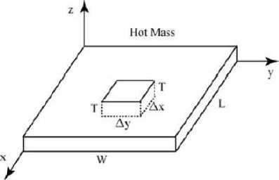
Fig.1. Cooling fin geometry [4]

Several methods have been developed aiming to overcome the numerical limitations imposed by the equation. The main techniques rely on converting the associated partial differential equation into a system of linear equations which may be solved by a mathematical software. Nonetheless, it is no rare that to build such a linear system constitutes the bulk of effort employed by modeling problems like the cooling fin one [5]. Moreover, the accuracy of those built models is commonly related to the precision into describing the temperature distribution along a fin surface which must be validate. Since this validation depends on incorporating well-known problem instances into the mathematical model for purposes of analysis, such a step requires an additional modeling effort which is generally prone to error.

This paper presents a simple and succinct modeling approach for the cooling fin problem. Both mathematical model and computational implementation offer a baseline which may be used as reference for the building of more complex scenarios as well as for validating additional tests instances of the problem. Therefore, the main contributions of this work are:

• •    A straightforward mathematical model for the cooling fin problem based on the finite differences numerical method.

• •    A flexible and efficient computational implementation of the proposed model on a free mathematics-oriented programming platform.

• •    An accuracy validation of the model through different instances of test which were evaluated on multiple levels of precision (meshes granularity).

The rest of this paper is organized as follow. Section 2 reviews the literature related to solving cooling fin problems. In Section 3, the mathematical model based on the finite differences numerical method is described for the cooling fin problem in a rectangular domain. Section 4 is dedicated to detail the computational implementations. Section 5 presents experimental results validating both model and implementation considering the solutions accuracy and the performance of the algorithm. Conclusions and directions for future work are included in Section 6.

• II. Related Work

The widespread use of fins in different applications has leveraged the proposition of many distinct approaches aiming to achieve models able to simulate the heat propagation as faithful as possible. An important contribution to solving the problem in a restricted rectangular domain was given by [6]. By studying the problem with variable heat transfer coefficient, the authors showed solutions for tip boundary conditions of constant heat flux and constant temperature. Thermally non-symmetric rectangular fins were explored by [7]. They described a reverse relation between a non-linear root temperature and the rate of heat loss from a fin. Considering extended general surfaces, [8] analyzed a set of distinct approaches for linear and non-linear situations. Some of those techniques are complex combinations, Laplace transforms, finite differences, finite elements, and boundary elements.

Besides the problem restricted to a rectangular shape, a variety of other works have addressed distinct geometry of domains. Analytical solutions for cylindrical pin fins were studied by [9]. The authors explored the method of separation of variables and examined the effects of tip convections on the temperature distributions along the entire fin and the heat flow rates at the fin base. Spiral fins were also analyzed by [10]. In this work, transient solutions of the temperature distribution and the heat flux at the base of the fin were achieved through Laplace transforms. Related to circular fins, [11] presented results when there are sinusoidal changes in the fluid temperature, and also when the fin is subjected to linear and higher order changes of fluid temperature. Another embracing study considering multiple fin shapes was conducted by [12]. Numerical solutions were shown for three types of fins combined with other three types of shapes. The results were evaluated according to four different initial conditions.

Alternatives technique have also been employed so that obtaining accurate solutions for cooling fin problems. Working around the additional effort associated to the validation of solutions obtained from numerical methods, [5] validated the developed analysis of rectangular fins by means of ANSYS® programming software [13]. Another approach focused on the heat conduction in tapered cooling fins was presented by [14]. The authors applied symbolic programming techniques to model the heat conduction in fins with triangular profiles. In such a work, they presented numerical solutions which fast converge to the corresponding analytical solutions. Employing calculus of variations, [15] published solutions for a rectangular fin submitted to zero surrounding temperature.

As a last related work to be cited, the transient analysis of two-dimensional cylindrical fin published by [16] presented an analytical solution for the cooling fin problem with various surface heat effects. The temperature distribution and heat rate transfer were generalized for a linear combination of the product of Bessel function, Fourier series and exponential.

III. Finite Differences Method in a Rectangular Domain

A traditional manner to solve partial differential equations is by the discretization of their domain. This process requires a PDE be approximated by equations with a finite number of unknowns. Such a discretization makes a PDE feasible to be solved by a computer [17]. A straightforward tool for the definition of approximations for partial derivatives in a PDE is taking their Taylor series expansion. Taylor series are able to describe how the information about a function at a point x may be used to evaluate such a function around the neighborhood of x [18].

As described by [19], a rectangular domain

Q = {(x, y), a < x < b, c < y < d} may be discretized as follow.

,   ( b - a )

h x =-- > X i = a + ( i - 1) h x ,    i = 1,..., n      (5)

( n - 1)

Using first and second order approximations, the replacements which must be done in a partial differential equation should corresponds to equations (7), (8), (9), and (10), where ®( h 2 ) and ®( h ) are related to the truncation errors [20].

d u /      ,

—⁽ x i , y) = d x

U i + 1, J - U i - 1, J

2 h x

Ui + 1 - Ui - 1

2 h x

d u

—⁽ x i , y) = d y

, ® ( h ')

U i , J + 1 - U i , J - 1

2 h y

Ui + n — Ui - n

2 h y

, ® ( h ²)

⁽ d  c )

h y = ------^ y J = c + ( J - 1) h y , J = 1,..., m    (6)

( m - 1)

d U ,      , U i - 1, J - 2 U i , J + U i + 1, J

— (xi, yi) =-------------------- dx                 h2

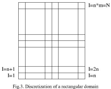
Such a discretization makes possible each point u(x_i, y j ) of a function u defined in a rectangular domain Ω, be approximated by linear equations. In this work, the approximation of a point u(x i , y j ) will be denoted by u i,j . For simplification purposes of notation, each point (i,j) of a mesh that discretizes a rectangular domain Ω will be rewritten as one-index dependent. Fig.2. depicts the mapping of coordinates assumed for each mesh point. Based on this new notation, the discretization of a rectangular domain Ω may be seen as described by Fig. 3.

ui - 1 - 2 u, + ui + 1

--------7^--------, ®⁽ h x )

hx

d U             U i , J - 1 - 2 U i , J + U i , J + 1

—(x, yi) =----------------- dy                 hy

Ui - n - 2 U, + Ui + n -------72------- , ® ⁽ h_y)

Applying such approximations in the transport

equation (1), equation (11) is obtained

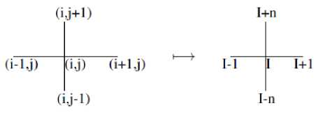
Fig.2. Mesh points redefined as one-index dependent

^d I ^U I - N ^{+ b} I ^U I - 1 ⁺ a I ^U I ^{+ C} I ^U I + 1 ⁺ e I ^U I + N    fl

I <  I <  N = m • n

with the corresponding coefficients

d, =- k - ^^

^I    h y ²    2 h y

^I    h x ²   2 h x

- k в

^I h x ²   2 h x

- k в e, =—r + — I    hy2   2hy

⁺ Yi

Two types of boundary conditions were implemented in this work. The first one involves the definition of prescribed values for the boundaries of the domain. As the analyzed problem is related to a rectangular domain, this scenario requires that four values are provided for the four respective limits. Moreover, the coefficients of

where m and n correspond to the number of discretization points in the directions x and y respectively. Considering equation (4), which describes the cooling fin problem, the coefficients generated by the finite differences method – equation (11) - should be rewritten as follow.

equation (11) must be modified as follow.

a^a = 1(20)

d^d = 0(21)

biWbi = 0(22)

c^c = 0(23)

fH f = prescribed value(24)

— k

b_T = c

— k

¹ = h

a_x = 2 k

11 h?⁺h !

2 c

T

The approximations obtained from the finite differences method generate an A pentadiagonal matrix of a linear system Ax = B as described by Fig. 4. The solution of such a linear system results in a numerical solution of the cooling fin problem.

<71 С]               C1

Ь?   Gi C₂

dn-V\ ^«+1 ^n+l di

^2

cn+l       ^+1

bl     ai     Ci dN-\       bN-\  gn-\ dN        bN

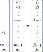
Fig.4. Pentadiagonal linear system generated by the finite differences method.

IV. Implementation

Algorithm 1 (Fig. 5.) details the steps implemented for solving the cooling fin problem (CFP). Lines 3 and 4 define the granularity of the mesh to be used by the algorithm. The main loop (lines 6-16) is responsible for building both the pentadiagonal stiffness matrix A and the vector of independent terms ( F ). Boundary conditions (Line 17) are set by an additional procedure.

Algorithm 1 Finite Differences Algorithm for the CFP Input: Integer с, T, L, W, u_re^ K_t nnodes_x, nnodes_y Output: Array of temperatures x

• I:    Pv = Py = 0;

• 2:    y= 2*c/T;

• 3:    h_x = L/(nnodes_x — 1);

• 4:    h_y = Ж /(nnodesy - 1);

• 5:    Build two-dimensional mesh;

• 6:    foreach (node n : meshing) { // Stiffness matrix A

• 1:    aj(n) = у+2^*(1/А^ + 1 /h^y,

• 8:     d =bi = -K/h²_x;

• 9:    4(n) = г/(л) = -K/h^;

• 10:    А(н_?п) = л/;

• 11:    А(п_?н + 1) = с/;

• 12:    A(n,n-l) = fr/;

• 13:     A(n,n-Vnnodes_x^ = ei;

• 14:    А(л,л — nnodesx') = df,

• 15:    F(n) = y*u_re/;

• 16:    }

• 17:    Set boundary conditions;

• 18:    Solve linear system Aa = F;

• 19:    returns;

Fig.5. Finite Differences Algorithm for the CFP

Algorithm 2 (Fig. 6.) describes the auxiliary procedure used for setting such prescribed values. This procedure should be invoked by Algorithm 1 during the step of boundary conditions definition (Line 17).

Mixed boundary conditions constitute another type of cooling fin problem evaluated in this work. In this scenario, there is a known linear relation between the function u and its derivative, which is described by equation (25).

V d n ) i

Algorithm 2 Prescribed Value of Boundary Conditions for the CEP_________________________________________

Input: A,F, nnodes.L,W,KJival,lvaLrval

Output: Matrix A

• 1:    foreach (int n : nnodes) {

• 2:     if (n e [x,0] boundary)

• 3:         value = dval;

• 4:     else if (n e [x^] boundary)

• 5:          value = uval;

• 6:      else if (n e [0,y] boundary))

• 7:          value = Ival;

• 8:      else if (n e [L,y] boundary))

• 9:         value = гш/;

• 10:     А(л,:) = 0;

• 11:     A(n,n) = 1;

• 12:     F(n) = value;

• 13:    }

• 14:    return A;

Fig.6. Prescribed value of boundary conditions for the CFP

Since a rectangular domain Ω has been considered, the derivative related to the exterior unitary normal is is defined as follow.

8 u d n

— du

-----, for I = 1,2,..., n dy du „ T „ .           .

—, for I = n ,2 * n ..... m * n dx

—, for I = ( m — 1) * ( n + 1),..., m * n d,

- du г. т i 1                      1

----, for I = 1, n + 1,...,( m — 1) * n + 1

I dx

c^c, = 0              (31)

f i^ = f, — C I h x q-          (32)

a ,

Algorithm 3 (Fig. 7.) describes the implementation of such changes in order to incorporate a mixed boundary condition in the cooling fin equation.

Algorithm 3 Mixed Boundary Conditions for the CEP

Input: A. F, h_x, h_y, nnodes,L,W,K.u_ref,c

Output: Matrix A

• 1:    foreach (int n : anodes) {

• 2:      if (n E [L,y] boundary)

• 3:      А(и,л)+=А(л,л+1)*(1 ~(h_x/K);

• 4:        F(^)+ = A(n,n + 1) * h_x/K * u_rej;

• 5:      А(л,л+1)=0;

• 6:      else if (n € [x,0] boundary))

• 7:       А(и,л)+ = A(n,n — 3) * (1 — (c^hy/K);

• 8:        F(a)+ = A(n,n — 3) *c*hy*u_rej/K;

• 9:       А(л,л —3) = 0;

• 10:      else if (n e [x,VV] boundary))

И:       А(л,л)+ = A(n,n + 3) ♦ (1 — (c*hy/K);

• 12:       F(«)+ = A(nji + 3) *c*hy *u_rej/K;

• 13:       А(л,л + 3)=0;

• 14:    }

• 15:    return A;

Fig.7. Mixed boundary conditions for the CFP

Depending on the position of I in the boundary, one of the variables I-n , I-1 , I+1 , I+n will be out of the domain. In this case, equation (11) should be modified. If I = 1, 2, …, n , the changes to be carried out on the equation are as follow.

a_T w aj = a _T + d.

fi M, ) 1

“ ,

fi^fi = fl — dI—q,        (29)

“ q

On the other hand, if I = n , 2* n , …, m * n , the modification to be applied on equation (11) are the following.

V. Experimental Results

The Octave scientific platform [21] was used for the implementation of the finite differences method. It is a high-level mathematical programming language which offers to the programmer a toolkit of implemented functions such as the linear systems solver employed in the proposed algorithm. The complete source code of the implementation was made available on a GitHub repository [22]. The experiments were performed on a PC running Ubuntu Linux, version 14.04.5 LTS, with Kernel version 3.19.0-31. It consists of one Intel i7-3610QM processor of 4 cores (two threads per core), operating at 2.3 GHz. Each core has a unified 256KB L2 cache and each processor has a shared 6MB L3 cache. The PC contains 8GB of main memory.

The two instances of the cooling fin problem analyzed in this work were proposed by [4]. They differ by the type of boundary conditions. The first one consists of setting up prescribed values for the boundaries of a rectangular domain (PVBC) as follow.

aj I—> aj = aj + c_z

fl   h x P , )

PVBC =

u ( x , 0) = u ( L , y ) = u ( x , W ) = 70 u (0, y ) = 200

Another considered instance of the problem involves mixed boundary conditions (MBC), that is, there is a heat flux at a tip of the rectangular domain. The setting up of such a scenario was modeled by conditions (34). Complementary to the definition of those boundary conditions cases, the dimensionless physical parameters proposed by [4] were also configured into equation (4).

Such additional conditions are described in (35).

u ( x ,0) = u ( x , W ) = 70

MBC -^ u (0, y ) = 200

^{u (} L , У ) = - k ^ = c (^{u (} L , У ) - ^u ref ) d n

\ T - ²

^{L -} W ^{- 1}

< k - 1                                     (35)

^u rf ^{- 70}

^ c — 1 (heat transfer coefficient)

Different levels of discretization (meshes) were used in the numerical experiments. The granularity of employed meshes varied from 3x9 - the most coarse one - up to 129x33. The execution time achieved for different tested meshes is presented in Table 1. In a general way, solving both problem instances presented a similar performance for all tested meshes. Indeed, the most significant performance difference was observed with the 33x129 mesh, which was of just 29%.

Table 1. CPU time comparison: PVBC (Prescribed Values Boundary Conditions), MBC (Mixed Boundary Conditions)

Mesh size (nXm points)	CPU time (sec.)
	PVBC	MBC
3 x 9	0.012	0.013
9 x 3	0.016	0.017
5 x 5	0.015	0.016
5 x 15	0.053	0.051
15 x 5	0.052	0.051
9 x 9	0.057	0.053
9 x 31	0.207	0.180
31 x 9	0.201	0.197
17 x 17	0.197	0.184
17 x 65	1.206	0.939
65 x 17	1.213	1.228
33 x 33	1.045	0.930
33 x 129	30.582	21.714
129 x 33	33.693	29.946
65 x 65	24.830	23.482

Nevertheless, it was noticed a significant impact on the CPU time as the mesh granularity was refined. In fact, an about fourfold increase in the number of discretization points (from 33x33 to 33x129) yielded a CPU time increasing of 30X for the PVBC problem and of 21X for the MBC problem approximately. Moreover, for meshes with the same granularity but with distinct horizontal and vertical configurations of points, it was achieved different performance rates. An example may be seen with the meshes 33x129 and 129x33. With the first one, the solutions of both problems were obtained faster than with the second one. More precisely, there was a performance decreasing of 9.23% for the PVBC problem and of 27.49% for the MBC problem. On the other hand, such a performance compromising was not noticed with more coarse meshes.

In order to evaluate the quality of the solutions achieved for both PVBC and MBC problems, graphics were plotted for one of the most refined simulations -meshes of 65x65 points. Fig. 8. and Fig. 9. present the behavior of the transport equation in the context of the cooling fin problem. Different temperatures throughout the rectangular domain are depicted in the graphic by different colors.

Since there is no any external influence (heating flux) in the first problem instance (Fig. 8.), the temperature in the neighborhood near to the boundaries [x, 0], [L, y], and [x, W] is the same of the temperature of reference ( u ref = 70). Toward the tip [0, y], the temperature is ascending up to the original prescribed value for such a boundary.

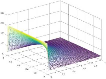
Fig.8. Temperatures from Prescribed Values Boundary Conditions

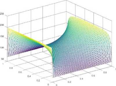
Fig.9. Temperatures from Mixed Boundary Conditions

In the mixed boundary conditions instance, there is a heat flux at the tip [L, y]. The influence of such a flux in the related area may be seen in Fig. 9. which depicts higher temperatures like ones observed at the boundary [0,

y]. The two other boundaries, that is [x, 0] and [x, W], are also affected by the external heat flux. Indeed, the regions nearby those two tips present temperatures higher than the observed in the same regions from the previous instance (PVBC).

• VI. Conclusion

This work presented an implementation of the finite differences method for the cooling fin problem in a rectangular domain. Two instances of the problem were analyzed. The first one considered prescribed values conditions in the four boundaries of the domain. The second instance was related to mixed boundary conditions, that is, a heat flux was assumed in one of the boundaries.

Considering the performance of the proposed implementation for solving the problems, there is no relevant difference between both instances. Nonetheless, the efficiency of the presented implementation degraded as the granularity of the employed meshes increased. In fact, the CPU time increased up to 30X for a corresponding increase of mesh of just 4X. Moreover, it was observed that to solve instances which employ meshes with more points in the direction X than in the direction Y are slower than ones employing meshes in reverse setting up (more points in the direction Y than in the direction X). Those two features of the proposed implementation for the finite differences method indicate that the step of solving the linear system resultant from the modeled cooling fin problem must be refined. Since it is the heaviest step of the presented algorithm, more efficient strategies for solve sparse linear systems represent a relevant future work.

Related to the quality of the achieved solutions, the plotted graphics endorse their accuracy. In fact, the developed model and its respective computational implementation were able to describe the temperature along the whole rectangular fin surface. Therefore, this work may be explored as a baseline for the modeling of other distinct and more complex scenarios related to the cooling fin problem.