An Iterated Function System based Method to Generate Hilbert-type Space-filling Curves

Published Online November 2015 in MECS DOI: 10.5815/ijitcs.2015.12.02

• I.    Introduction

  A space-filling curve is a continuous mapping from the unit interval onto the N -dimensional unit hypercube and passes through each point of the unit hypercube. In 1890, Italian Mathematician G. Peano surprised the mathematical world by his ingenious discovering a spacefilling curve of traversing points on a two-dimensional 3 n x 3 n square grid exactly once and without crossing the path [1]. By mapping each point in a N -dimensional space into a one-dimensional space, the complex multidimensional access method can then be transformed into a simple one-dimensional one. Hence a lot of research has been done and there exist many kinds of space-filling curves [2]. Among them, the Hilbert spacefilling curve, which is another space-filling curve presented by Hilbert to traverse points on a twodimensional 2 n x 2 n square grid, preserves point neighborhoods as much as possible [3]. Thus Hilbert space-filling curve is applied widely in digital image processing, such as image encoding, image clustering, image encryption, image storing/retrieving, and pattern recognition [4, 5, 6]. A mathematical and historical review of Hilbert space-filling curve applications can be

seen in [2] and the references therein.

Iterated function system, or IFS for short, is one of the most common techniques to generate fractals [7-9]. IFS plays an important role in fractal geometry and has been found to have potential in different fields of physics, engineering, biology, geology, finance, etc. It also has been shown good performances in computer graphics and image processing, especially in the simulation of nature landscapes and digital image compression [10,11]. In this paper, we will present an IFS based approach to generate Hilbert-type space-filling curves. We will explore the generation of Hilbert-type space-filling curves via iterated function system systematically. It is a simple vertices generator for two-dimensional Hilbert-type space-filling curves. Based on a recursive calling Hilbert original space-filling curve n — 1 , we can generate the vertices set for the considered Hilbert-type space-filling curve at any resolution n . We then get the Hilbert-type space-filling curve by connecting the yielded vertices orderly. Because the generation of Hilbert’s original space-filling cure is common and easy, other Hilbert-type space-filing curves can be easily produced by integrating the recursive calling procedure of Hilbert’s original space-filling curve at resolution n — 1 and an IFS consisting of four affine transformations. The merits of the proposed algorithm lie in two aspects. It is easy to implement recursively calling Hilbert’s original spacefilling curve and can be generalized to produce other variation versions of Hilbert-type space-filling curves. Furthermore, the generated vertices coordinates can be easily quantified and applied to translate the twodimensional gray values of digital images to onedimensional version. As a result, the proposed algorithm can be effectively employed for image processing, such as image compression and image encryption, etc.

The remainder of this paper is organized as follows. Section II introduces some recently related works on Hilbert space-filling curves. Section III presents an iterated function system based method to generate six Hilbert-type space-filling curve patterns systematically. Section IV describes the corresponding variation versions of Hilbert-type space-filling curves constructed in Section III. Section V draws some conclusions.

• II.    Some Related Works

Since the fundamental work of Hilbert in which he formulated curves that visit every point in a unit square, there have been many research works on how to formally specify the Hilbert space-filling curve using either an operation model or a functional model. There are many algorithms for Hilbert space-filling curves, such as the Butz algorithm [12], the Quinqueton algorithm [13] and the Agui algorithm [14]. However, these algorithms have more or less restrictions on their applications, and this makes them very difficult to be put in practice. For example, Butz computed the mapping function by bit operations such as shifting, exclusive OR, etc. The algorithm is complex to compute and is difficult to implement in hardware. Agui and Quinqueton used the recursive functions to generate the space-filling curve, and their algorithms were complex and took time to compute the one-to-one mapping correspondence. So their algorithms were very difficult to apply in real-time systems. To improve the scanning efficiency via Hilbert space-filling curve, Kamata et al. proposed a simple, nonrecursive algorithm for N -dimensional Hilbert spacefilling curve using lookup tables [15]. The merit of the algorithm is that the computation is fast and the implementation is much easier than previous ones. Similar techniques based on lookup tables are adopted by Zhang et al. [16]. Lin et al. proposed an algorithm to generate Hilbert curves by tensor product [17]. The tensor product formulas can be directly translated into computer programs and therefore it is simple and easy to manipulate. Liu presented four alternative patterns of the Hilbert curve in [18]. The four patterns presented, together with Hilbert’s original pattern [3] and Moore’s pattern [19], comprise a complete set of the Hilbert space-filling curve. Liu used a parameter called resolution to describe the domain granularity of the concerned curve, then constructed the Hilbert-type spacefilling curve patterns via generation of the configuration of considered pattern from resolution k to k +1. The generation is determined by some affine transformations which are expressed in complex variable. However the presented method is not practical as it does not give the operable algorithm.

• III.    Six Hilbert-Type Space-Filling Curve Patterns

Although the literature has almost exclusively referred to the original pattern discovered by Hilbert, there exist other five alternative patterns, including Moore’s in [19], L1-L4 mentioned in [18]. As a matter of fact, any one of the five alternative Hilbert-type space-filling curve pattern at resolution k consists of four half-size Hilbert’s original pattern at resolution k + 1 placed end-to-end with appropriate orientations. Set the unit square to be [ - 0.5,0.5] x [ - 0.5,0.5], we will express the Hilbert-type space-filling curves at this unit square by iterated function systems.

• A.    Hilbert’s Original Pattern

Hilbert’s original pattern starts at one corner of the unit square, for example, (-0.5, -0.5), and ends up at its adjacent corner, for example, (0,5,-0.5). Hilbert’s original pattern at resolution k +1 can be determined by its vertices, which can be derived from the pattern at resolution k by the following transformations:

1 f 0

1 f 1

1 f 1

1 f 0 2 1 -1

The matlab code to generate the Hilbert’s original space-filling curve by iterated function system (1) is outlined in function module hilbert(n), which may be called in the form “[x,y] = hilbert(n)”. x, y stand for the x-coordinate and y-coordinate of the vertices of Hilbert original pattern at resolution n respectively. The initial set is one single point set {(0,0)}. The corresponding Hilbert’s original patterns with any resolution can be generated by connecting the yielded vertices (x,y).

function [x,y] = hilbert(n)

if n <= 0

x = 0;y = 0;

else

%recursive call to get coordinates %at resolution n-1

[x0,y0] = hilbert(n-1);

%calculate coordinates at

%resolution n by (1)

x = .5*[-.5+y0 -.5+x0 .5+x0 .5-y0];

y = .5*[-.5+x0 .5+y0 .5+y0 -.5-x0];

end plot(x,y,'-');

• B.    Moore’s Pattern

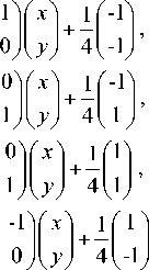
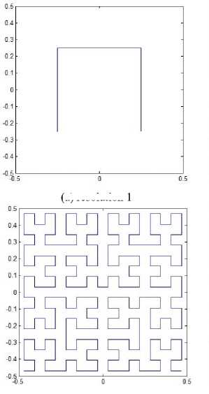
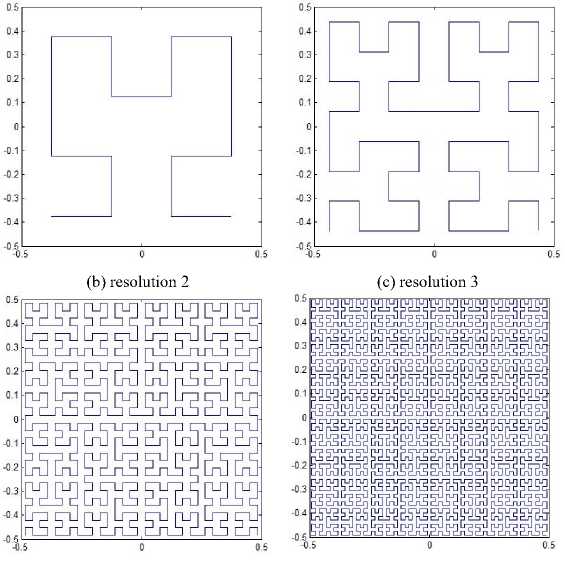
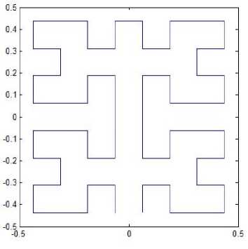
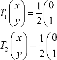
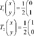
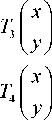
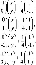
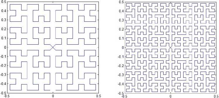
Moore reported an alternative Hilbert-type spacefilling curve pattern [19]. The graphical representation of Moore’s pattern of resolution 1 is the same as shown in Fig. 1(a), and the representations of resolution 2, 3, 4 and 5 are depicted in Figs. 2(a)-(d). Moore’s pattern starts at the midpoint of one side of the unit square, for example (0,-0.5), and ends up at the same point. As mentioned above, Moore’s space-filling curve consists of four halfsize Hilbert curves placed end-to-end with appropriate orientations. Thus, Moore’s pattern at resolution k+1 can be determined by its vertices, which can be derived from the vertices, of which the Hilbert’s original pattern at resolution k consists, by the following transformations:

T T1 1	x 1 . y )	2 (	0 1	01 )	f x 1 I y J	1 f —1 1 + 4 1 —J ,
T T2 [	x 1 . y J	" 2 1	0 1	-1 1 0 J	f x 1 I y J	\ + 4 f4),
T 3	f x 1 I y ,	1 = 2	f 0 I -1	1 1 0 J	f x I y.	J+ 4 f 1 ) ,
T 4	f x I y ,	I" 2	f 0 I -1	1 1 0 J	f x' I y,	I+ 4 f -1 ) .	(2)

The matlab code to generate Moore’s original spacefilling curve by iterated function system (2) is outlined in function module moore. It calculates and returns the coordinates of the nodes of Moore's space-filling curve pattern at resolution k . It also draws the curve at resolution k . Note that in this pattern, one can utilizes the vertices of the Hilbert original pattern at resolution k-1 . The matlab code to generate other alternative patterns is similar to that of Moore pattern.

function [x,y] = moore(k)

if k <= 0

x = 0; y = 0;

else

[x0,y0] = hilbert(k-l);

x = .5*[-.5-y0 -.5-y0 .5+y0 .5+y0];

y = .5*[-.5+x0 .5+x0 .5-x0 -.5-x0];

end plot(x,y,'-');

(d) resolution 4

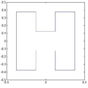
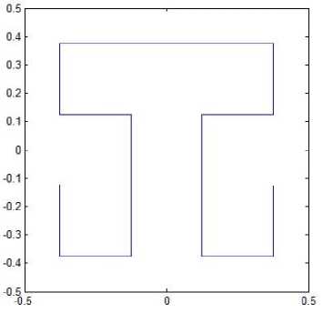
(a) resolution 1

(f) resolution 6

(e) resolution 5

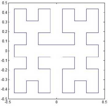
Fig. 1. Hilbert’s original patterns.

(b) resolution 3

(a) resolution 2

(c) resolution 4

(d) resolution 5

Fig. 2. Moore’s patterns.

C. Pattern L1

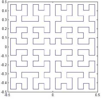
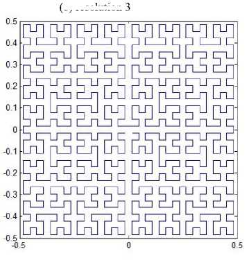
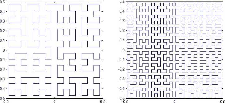
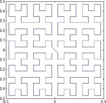
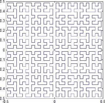
Suppose the space-filling curve starts at the center of the unit square and ends up at the same point. The graphical representation of resolution 1 for pattern L1 is the same as shown in Fig. 1(a), and the representations of resolution 2, 3, 4 and 5 are depicted in Fig. 3. Similarly, this space-filling curve consists of four half-size Hilbert curves placed end-to-end with appropriate orientations. Thus, one can apply the Hilbert’s original pattern at resolution k to generate this pattern at resolution k +1. The iterated function system is determined by

x10

T    = -           + -,

• ¹    ( y J  2 ( 0  -1 J( y J  4 ( -1 J

• x)   1Г0  -1)Гx)

"               + yJ 2 (1  0 J( yJ4

x)   1Г 0  1 )Г x)

"              + yJ  2 (-1  0 J( yJ4 x10x1

T    = -           + -    .

⁴ ( y J 2 ( 0  -1 J( y J  4 ( -1 J

E. Pattern L3

x )    1 ( -1   0Y x )    1 ( -1 )

=+ yJ  2 ( 0  -1J( yJ  4 (-1J x )  1 I1  0 V x)  1 I-1)

=+, yJ  2 (0  1 J( yJ4 x )_ 1Г1  0 )| x ) 1 f1)

yJ" 2(0 1J( y J + 4(1J , x-10

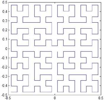
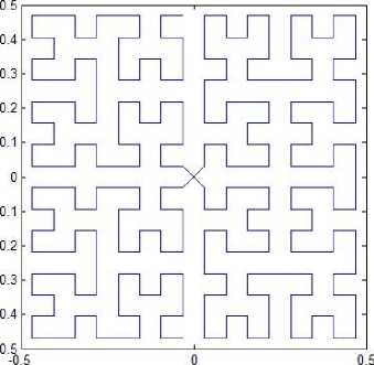
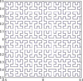
If the Hilbert-type space-filling curve starts at the lower left corner of the unit square and ends up at the center of the square, we can produce an alternative spacefilling curve whose four patterns for resolution 2 to resolution 5 are shown in Fig. 5. The pattern of resolution 1 is just the same as Fig. 1(a) for Hilbert’s original curve. The iterated function system is determined by

T     = -            + -    .

⁴ ( y J 2 ( 0  -1Д y J 4 ( -1 J

The matlab codes to generate L1 pattern and the rest patterns of Hilbert-type space-filling curves by iterated function system are similar to that of function module moore, and so we omit the their corresponding matlab source codes.

D. Pattern L2

x 1

T    =

• ²    ( y J 2 ( 0

_т Г x )₌ - г ¹

• ³    ( y J 2 ( 0

x -1

T    =4    I I                  I

( y J 2 ( 0

1 II x)   1 Г-1)

+

0 J( y J   4 ( -1 J

0 )I x )

+

1 J( y J   4 ( 1 J

0 Y x )

1 J( y ^{J +} 4 ( 1 ^J ,

0II x)

JI J +I J.

-1 J( y J  4 ( -1 J

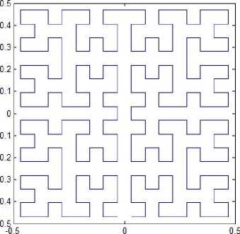
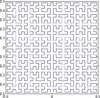
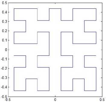
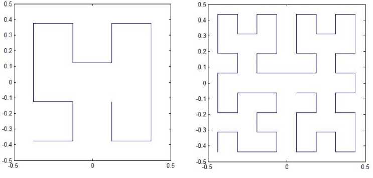
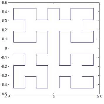
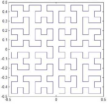
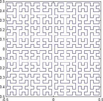
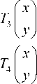
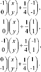
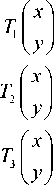
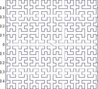
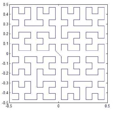
Suppose the pattern curve starts at the midpoint of one side of the unit square and ends up at the midpoint of the opposite side. This yields a new space-filling curve whose four patterns for resolution 2 to resolution 5 are shown in Fig. 4. The graphical representation of resolution 1 for pattern L2 is the same as Fig. 1(a). The iterated function system is determined by

F. Pattern L4

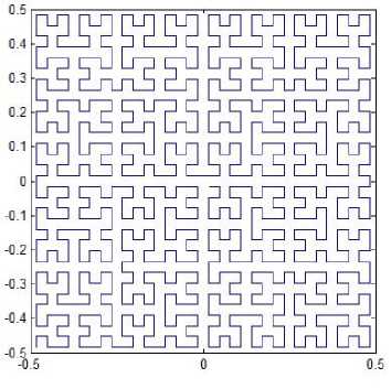
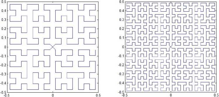
Let the Hilbert-type space-filling patterns curve starts at the midpoint of one side of the unit square and ends up at the midpoint of its adjacent side. One can generate a new space-filling curve whose four patterns for resolution 2 to resolution 5 are shown in Fig. 6. The iterated function system is determined by

т

T ₂

( : : 2 : 0 я :  .

T31 у ) 21-1 0 А у) + 411J ’-■О-11:: i:'-4 И

(a) resolution 2

(b) resolution 3

(c) resolution 4

(d) resolution 5

(a) resolution 2

Fig. 3. Pattern L1.

(b) resolution 3

(c) resolution 4                              (d) resolution 5

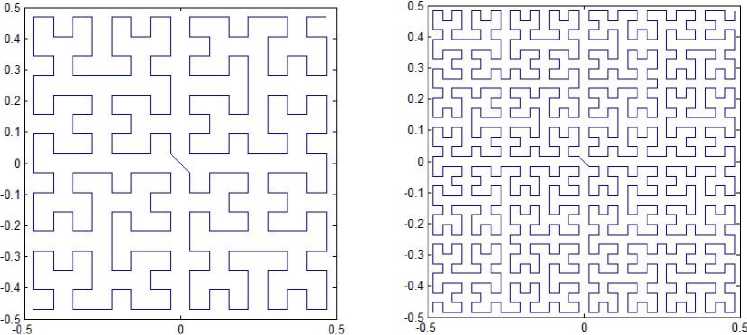
Fig. 4. Pattern L2.

(b) resolution 3

(a) resolution 2

(c) resolution 4

Fig. 5. Pattern L3.

(d) resolution 5

(b) resolution 3

(a) resolution 2

(c) resolution 4

Fig. 6. Pattern L4.

(d) resolution 5

IV Some Variation Versions of Hilbert-type Spacefilling Curve

A. Variation of Hilbert’s Original Pattern

As mention in Section III, Hilbert’s original pattern starts at one corner of the unit square, for example (-0.5, -0.5), and ends up at one of its adjacent corners, (0.5,-0.5) for example. To get a variation version, we change the end point to be (0.5,0.5), that is, the space-filling curve is from one corner of the unit to the opposite corner instead of the adjacent corner. We can also get a space-filling curve and the iterated function system is determined by

B. Variation of Moore’s Pattern

Let the space-filling curve starts at the midpoint of one side of the unit square, for example (0, -0.5), and ends at the same point. Meanwhile, the curve passes through center of the unit square two times from which the Moore’s pattern is different. We can also get a spacefilling curve. The iterated function system is defined by

x 0

T= -

I У J 2 1 ¹

x1 T=

21 y J2

т Г x)- Г

31 y J 2 ( 0

1 Y x)

+

0 J( y J 4 ( -1 J

0 Y x ) 1 Г -1 )

1 JI y J ⁺ 4 1 1 J ’

0Yx)

• -1 J( y J⁺ 4 ( -1 J ,

• -1Y x )

+

0 JI y J 4 1 1 J

x 0

Tx\    1 = -I

( y J 2 ( 1

x 0

T2|=

I y J x0

T=

³ ( y J 2 ( -1

x 0

T =-

T4 \ I y2-1

-1 )Г x )   1 Г -1

+

0 Л у J  4 ( -1

0 J

x 1

y ) + 411)

-1)Г x)

+

0 Л y J 4 (1

1)Гx)

+

0 Л y J4

C. Variation of Pattern L1

Suppose the space-filling curve starts at the center of the unit square and ends at the same point. However the curve is different from pattern L1. We can also get a space-filling curve with iterated function system

T V	x ) . У У	2 (	-1 0	0 ) -1 J	Г x V У У	)+ 1 1	г -1 ) v -1 J ’
T 2	Г x ' 1 У у	1 • 2	Г 1 1 0	0 1 У	Г x 1 V у У	• 4 1	-1 ) . 1У ,
Т 1	' * ) v У У	■ ’ 1	1 0	0 ) -1 J	Г x V У У	1 !• 4 i	1 ) -1 J ,
T 4	Г x 1 1 У У	1= 1 1	г -1 v 0	0 ) 1 У	Г x V У У	)• 4 1	Г 1 ) v 1 J .	(9)

1 Г -1 0 Y x )

2 1 0  1 Л У У

1 Г1)

• .

4 (1J

D. Variation of Pattern L2

F. Variation of Pattern L4

Suppose the curve starts at the midpoint of one side of the unit square and ends up at the midpoint of its adjacent side. But it passes the center two times from which pattern L4 is different. This yields a new space-filling curve whose two patterns for resolution 4 and resolution 5 are shown in Fig. 12. The corresponding iterated function system is defined by

Suppose the curve starts at the midpoint of one side of the unit square and end up at the midpoint of the opposite side and the curve pass through the center two times. This yields a new space-filling curve whose four patterns for resolution 4 and resolution 5 are shown in Fig. 10. We can get a variation version of pattern L2 with iterated function system

1 г -1 2 V 0

1 Г о 2 1 1

1 Г 0 2 1 -1

1 Г 1 2 V 0

E. Variation of Pattern L3

Suppose the curve starts at the lower left corner of the unit square and ends up at the center of the square, but this time the curve passes through alternative way different from L3. This yields a new space-filling curve whose two patterns for resolution 4 and resolution 5 are shown in Fig. 11. We can get a variation version of pattern L2 with iterated function system

1 Г о 2 1 1 1 г 1 2 V 0 1 г 1 2 V 0

1 Y x 1  1 Г-1)

•, о )( y J 4 (-1J

0Yx) 1 Г-1) 1Л y J + 4 ( 1 ] ,

0)Гx)  1Г 1)

-1 JI У J+ 4 ( -1 J ,

V. Conclusions

Hilbert-type space-filling curve has attracted much interest thanks to its mathematical importance and extensive applications in signal processing, such as encoding, image clustering, encryption, image storing/retrieving, and pattern recognition, etc. Besides the original one discovered by Hilbert himself, there exist other patterns. Moore presented such a pattern in 1900. Liu explored other four alternative ones in 2004. In this paper, we construct the six patterns form an iterated function system point of view. The constructed iterated function system for the considered pattern can be easily generated by cooperating a recursive calling the common Hilbert original space-filling curve and IFS consisting of four affine transformations. It is then easy to depict the pattern and to be applied to image processing. Besides the six Hilbert patterns mention in [18], we construct their corresponding variation versions thoroughly as well. The applicability of all these Hilbert-type patterns may be paradigm-dependent. For example, the finite-elementmethod in electromagnetic field analysis would benefit from a particular pattern, since there are various boundary conditions that may make sense to wrap around the finite grid in defining a region.

(a) resolution 4                              (b) resolution 5

Fig. 7. Variation of Hilbert’s original patterns.

(a) resolution 4                              (b) resolution 5

Fig. 8. Variation of Moore’s patterns.

(a) resolution 4

Fig. 9. Variation of Pattern L1.

0.5

-0.51--------------------------------------------1--------------------------------------------

-0.5                             0                            0.5

(b) resolution 5

(a) resolution 4

(b) resolution 5

(a) resolution 4

Fig. 11. Variation of pattern L3.

Fig. 10. Variation of pattern L2.

(b) resolution 5

(a) resolution 4                              (b) resolution 5

Fig. 12. Variation of pattern L4.

Acknowledgment