An Iterative Technique for Solving a Class of Nonlinear Quadratic Optimal Control Problems Using Chebyshev Polynomials

Published Online May 2014 in MECS

Many direct methods have been developed to solve the nonlinear optimal control problems. All direct methods are based on converting the dynamical optimal control problem into static optimization problem, These methods are either based on discretization [1,2] or on parameterization. The parameterization can be implemented by parameterizing the state variables [3-5], control variables [6,7] or both the state and control variables [8,9].

Jaddu [3-5] proposed a method to solve the nonlinear optimal control problem using the quasilineraization and the Chebyshev polynomials. In [10-14] Banks and his coauthers developed a method to deal with the nonlinear systems by means of iterative approach.

In this paper, we propose a new method based on the Banks iterative technique to replace the nonlinear optimal control problem by sequence of linear time-varying quadratic optimal control problems. Then each of these problems is converted into quadratic programming problem. To this end, the Chebyshev polynomials are used to approximate the state variables. The proposed method in this paper is classified as a direct method. Approximating the state variables has the following advantages [3]: (1) There is no need to integrate the system state equations as in control parameterization. (2) The number of unknown parameters is smaller compared with control-state parameterization. (3) The state constraints can be handled directly; an example of this in this work is the approximation of the initial condition vector.

This paper is organized as follows: In section 2, the problem treated in the paper is stated. Section 3, shows how to apply the Banks iterative method on the problem of section 1. Section 4 describes the state parameterization and the approximation by Chebyshev polynomials. In addition, this section, shows the transformation of the dynamic optimal control problem into quadratic programming problems. Section 5 shows the simulation results of the Van der Pol oscillator optimal control problem and compares the results obtained using the proposed technique with other techniques. In section 6 some conclusion remarks are presented.

• II.    Problem statement

The optimal control problem treated in this paper can be stated as follows: Find an optimal controller и ∗ ( t ) that minimizes the following performance index

J=∫>tf (x тQx+uт Ru)dt (1)

subject to the constraints of the system state equations and initial conditions given by,

̇=А(X)X+В(X)и X(0)=х0 (2)

where Q is a positive semidefinite matrix, R is a positive definite matrix, х ∈ RH is the state vector, u ∊ R^m is the control vector, %о ∈ R¹¹ is the initial condition vector.

This problem will be solved by converting the nonlinear quadratic optimal control problem into a sequence of quadratic programming problems, which are easier to solve. The solution is based on using the iteration technique, which will replace the nonlinear quadratic optimal control problem into equivalent sequence of linear time-varying quadratic optimal control problems. Then, each of these problems will be solved by converting it into a quadratic programming problem by using state parameterization via Chebyshev polynomials.

• III.    Banks Iterative Technique

In this section, the iterative technique developed by Banks [10-14] is applied on the problem (1)-(2) to convert this problem into a sequence of linear time-varying quadratic optimal control problems as follows:

For i=0

Minimize j [о] = y£/(x[0]T Q x[0] + и^Т R u[0])d t(3)

subject to the following state equations and initial conditions

x[0] = Л(х0)х[0] + B(x0 )u[0]    x[o](0) = x0

and for i > 1

Minimize

J[t] = Jo£/(x[l]T Q x[l] + u[l]TRu[l])d t(5)

subject to the following state equations and initial conditions

• x^[l] = А (x ^{[l _ 1 ]} (t)) x ^[l] + В (x ^{[l _ 1 ]} (t)) u ^[l]

x [/](0) = xo

Each of the linear time-varying quadratic optimal control problem (3)-(6) is converted into a quadratic programming problems by applying the state parameterization technique using Chebyshev polynomials. Therefore, the time interval t £ [0, t y ] should be changed to т £ [-1,1] because Chebyshev polynomials are orthogonal when defined of the interval т £ [-1,1]. This will transform the problems (3)-(6) into

For i=0

Minimize

• J[0] = 77 jP/x10^ Q x[0] + u[0]TRu[0])dT

subject to:

dx ^[0]

• —7— = у рЦхо^⁰] + B^Xq №^]]

x [o](-1) = xo and for > 1

Minimize

J[t] = 77 L>MT Q x[l] + u[l]TR u[l])d т subject to:

[]

• —   = у *А (x ^{[l _ 1 ]} (т)) x ^[l] + В (x ^[l“ ^{1 ]} (t)) u^[i] j,

x [/](-1) = x0

• IV.    Chebyshev Approximation

To convert each of the optimal control problems (7)(10) into a quadratic programming problem, a set of the state variables are approximated by a finite length Chebyshev series with unknown parameters. Then, the remaining states and control variables are determined as a function of the unknown parameters of the approximated state variables from the state equations (8) and (10). In [15] a detailed description of how to apply the state parameterization using Chebyshev polynomials is presented.

Applying the method described in [15], the state variables can be approximated by using the Chebyshev polynomials of the first type as follows

U)

Xj = ^ + X N ^ТХт) j = 1,2 n (11)

where N is the length of the approximated series which depends on the required accuracy; large values of N yield good accuracy at the expense of computational time and vice versa, ai are the unknown parameters and Ti is a first type Chebyshev polynomial of order i . The control variables are obtained from the system state equations as a function of the state variables unknown parameters. These control variables can be rewritten in terms of a finite length series of Chebyshev polynomials with unknown parameters as follows

• и , = pp + a t 1 &P ) ^(r) l = 1,2 m (12)

where the unknown parameters b ^(Z) are function of the state variables unknown parameters a ⁽⁷ ) .

In state parameterization, it is necessary to obtain the derivative of the state variables. This can be done using Chebyshev polynomials differentiation properties as follows [16]

Л/(т)=^+Й'="11ад(т) j = 1,2.....n     (13)

where

( Q-n- 1 = 2Nd^

d_N - ₂ = 2(N - 1)d N-1                       (14)

a_r _ ₁ = a_r+1 + 2ra_r , r = 1,2, .„, N - 2

Equation (10) shows that the two matrices Л (x ^{[l 1 ]} (t)) and ( ^{[ ]} ( )) are a function of , therefore it is necessary to express every element in both matrices in terms of a Chebyshev series of known parameters. To this end, let Л ,-_; (т) = g(x ^{[l- 1]} (т),т) be the (j, Z) element of the matrix X(x ^{[l - 1]}(t)) where x ^{[l- 1]}(t) is the nominal trajectory of the previous iteration. Then the term Л у _г(т) can be expressed in terms of a Chebyshev series of known parameters of the form [16]

А / (т)=^ + 1Г = 1^(т)                (15)

where

Wj =-У ^(cos^ i )) cosset)

j = 0,1,^,N                       (16)

and 9t =     ,i=1,2,…,К and К>N (in this work we arbitrary set К=  +5). The same approximation can be done for the matrix 5(x[i"1](r)) .

Also equation (10) shows that Л(х[Н1](т)) , В(х[Н1](т))are time-varying matrices expressed as a function of Chebyshev polynomials of the previous iteration. The matrix Л(х^-1](т)) is multiplied by X , which is also expressed in terms of Chebyshev series with unknown parameters, and the matrix 5(х[Н1](т)) is multiplied by u[L] , which is also expressed as a function of Chebyshev series with unknown parameters. Therefore, it is necessary to have a multiplication algorithm to multiply Chebyshev series. This algorithm is given as follows [3]:

Given two Chebyshev series

X =∑ i=o Х[Т[                               (17)

Substituting (25) into equation (7) (for the first iteration) or equation (9) (for the next iterations), we get

^̂ J ^[ ‘] ₌^ ∫ 1 (Т тSi^TQS ! Т+ТTS2^TRS ₂Т)dτ      (26)

where ̂[1] is the approximated value of J at iteration i. By letting M=       and p=       and noting that both matrices M and p are symmetrical, Jaddu [3,15] derived an explicit formula for the approximated performance index ̂[1] given by,

̂ [ ¹]₌ tf ^∑ ^"l^{1 k}2 ( ́ i , i+k + ́ li , i+k )( ₍21-2H ) ⁺

)                             ( where pi,i+k k≠0

,   k=0

mi,i+k k≠0

mii      =

ṕ i,i+k={

Ү=∑“о ^у jТ                             (18)

ḿ i,i+k ={

Then the multiplication of these two Chebyshev series is a Chebyshev series of length n+m given by

∑n+m - гр

∑

where

where к = 0,2,4, ...,N (N even)or N — 1(W odd) and PiJ , ^mij are the elements of the symmetrical matrices p and M respectively.

The performance index in (27) can be rewritten as,

Zk _{= ∑} ^oXiVk-t ⁺ Xtyt-k ⁺ Х[У₁₊к          (20)

The next step is to approximate the initial condition vector x(-1)= x 0 and since we are using state parameterization, this task becomes very easy. By substituting т =-1 into (11) and using the following Chebyshev initial value property [16],

J 2

where

^п(-1) = (-1)71                                (21)

the initial condition vector is approximated as follows

( )^-а⁽¹ ) ₊ Cl ^{( 1 )} - ⋯ +(-1) ^Na ⁽; - ^xj (-1) =0 (22)

The last step is to approximate the performance index J . To do this, (11) and (12) are rewritten in matrix form

T   (1)(1)(1)(2)(2)(2)(z)(z)

а =[а     …а        …а …а …а]

is the unknown parameter vector and н is a ppositive definite [3] Hessian matrix given by

______52 ̂ dci ( "к ) до.( "к )

where i,j = ОД,..., N and к = 1,2, ... ,z . z is the number of directly approximated state variables.

The original nonlinear quadratic optimal control problem can now be restated as follows:

rxq

*2

Лг-

0.5а ⁽ ) ( ⁾ _⎢ ⎢⎢ 0.5 _⋮ ( ⁾ “ ( _⋮ ⁾ ⎣ 0.5а ⁽„^{) (} „ ⁾

1 Т min_a -а¹ На

subject to

Ui -u2

0.5b( )    b()

⎢0.5ь( )    b()

⎢⋮

⎣ 0.5 b ^(m) b ⁽ m ⁾

⁶⁽ ‘ ) _⎤ ^{6 (} _⋮ ^{! )} ⎥ ^⎥ h ⁽ m ^{) U}N ^J

[ : ⋮]

or in compact form

X ^[1] ₌ S-.T и ^[1] ₌ S₂T

F_ia =                                       (33)

where the equality constraints are due to initial conditions and in some cases unsatisfied state equations.

The standard quadratic programming problem (32)-(33) can be solved using any available software package.

To solve the original nonlinear problem (1) -(2), we need to solve time-varying linear quadratic optimal control problem (7)-(10) iteratively until

| ; ̂[i+1 ^] - ̂^[1]| _< е                                              (34)

is satisfied. In this work we consider 6 =10 ⁵.

• V.    Computation Results

• • Van der Pol Oscillator

Find an optimal controller        that minimizes the following performance index

J =1 fc2 + x2 + u 2 )d t(35)

subject to

%1 = %2    ,X1(Q) = 1

x2 = -x1 + (1 - x))x2 + u ,x2(0) = 0

Using the technique in sections 3 and 4, the problem can be reformulated as:

for i = 0

Minimize

J                                             t(38)

subject to

• ij0 l = x2[0 ]    ,xj0 ](0) = 1

• %2 [0] = —x1[0] + u[0]   ,x2[o](0) = 0

and for i > 1

Minimize

• J 'ЧЖ + ^Л* t(41)

subject to

^^] = x2[l ]    ,x1[l](0) = 1

x₂^[l] = -x- L^] + (1 — (x^[l " ^1] ) )x₂ ^[l] + u ^[l]

x2 [/](0) = 0

After changing the time interval            to the interval              ,        is approximated by a 9th order Chebyshev series, is determined from (42) while is determined from (40). The obtained values of xj_(t), x2(t) and u(t) of the first iteration are substituted into (42)-(43) to solve for the next iteration, after approximating x1(t) by 9th order Chebyshev series,

• ( ) and ( ) are obtained from (42) and (43) respectively.

Table 1 illustrates the results of the optimal values of the cost function verses iteration i for Chebyshev polynomial with N = 9 and N = 15. Table 2 shows the optimal values obtained using some other methods for comparison purposes.

• Fig. 1 shows the optimal trajectories of the Van der Pol oscillator problem.

Table 1. approximated optimal value

iteration i	N = 9	N = 15
0	0.9533622676	0.9533622624
1	1.4516540238	1.4515286014
2	1.4497313124	1.4496981112
3	1.4493918353	1.4493287644
4	1.4494606241	1.4494047276
5	1.4494528889	1.4493959719

Table 2. values of J obtained using other methods

Source	J	Method
Jaddu [3]	1.433487	Quasilinearization and state parameterization
Bullock and Franklin [17]	1.433508	Second variation
Bashein and Enns [18]	1.438097	Quasilinearization and discretization

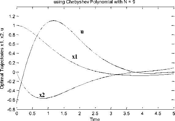
Fig. 1. Optimal trajectories of Van der Pol problem using Chebyshev polynomials

• VI. Conclusion

In this work, a method for solving a class of nonlinear quadratic optimal control problem has been proposed. This method is based on replacing the nonlinear state equation by a sequence of linear time-varying state equations and then parameterizing the system state variables by a finite length Chebyshev series with unknown parameters.

To show the effectiveness of the proposed method, a Van der Pol oscillator problem is solved and the simulation results obtained indicate that the proposed method gives good and comparable results with some other methods.