An univariate feature elimination strategy for clustering based on metafeatures

Автор: Saptarsi Goswami, Sanjay Chakraborty, Himadri Nath Saha

Журнал: International Journal of Intelligent Systems and Applications @ijisa

Статья в выпуске: 10 vol.9, 2017 года.

Бесплатный доступ

Feature selection plays a very important role in all pattern recognition tasks. It has several benefits in terms of reduced data collection effort, better interpretability of the models and reduced model building and execution time. A lot of problems in feature selection have been shown to be NP – Hard. There has been significant research in feature selection in last three decades. However, the problem of feature selection for clustering is still quite an open area. The main reason is unavailability of target variable as compared to supervised tasks. In this paper, five properties or metafeatures like entropy, skewness, kurtosis, coefficient of variation and average correlation of the features have been studied and analysed. An extensive study has been conducted over 21 publicly available datasets, to evaluate viability of feature elimination strategy based on the values of the metafeatures for feature selection in clustering. A strategy to select the most appropriate metafeatures for a particular dataset has also been outlined. The results indicate that the performance decrease is not statistically significant.

Еще

Feature Selection, Feature Elimination, Entropy, Skewness, Kurtosis, Coefficient of Variation, Correlation

Короткий адрес: https://sciup.org/15016423

IDR: 15016423 | DOI: 10.5815/ijisa.2017.10.03

Текст научной статьи An univariate feature elimination strategy for clustering based on metafeatures

Published Online October 2017 in MECS

Feature selection is one of the most important preprocessing tasks in any data mining, machine learning, and pattern recognition process. This has several benefits like [1][2][3] – reduced data collection effort, reduced storage cost, lesser model building and execution time and better model interpretability. The interpretability of the model is a key requirement and this is one of the reasons why feature selection is often preferred over dimensionality reduction methods like Principal

Component Analysis, Factor analysis etc. where the original features are transformed to generate new set of features and semantics of the features are lost [2][4]. The problem of feature selection is very relevant with the advent of Big-data, as the dimensionality of the datasets have increased significantly.

Feature selection for classification is relatively well defined, as the relevance of a feature can be estimated by its ability to predict the target or the class variable [24][25]. In case of clustering the problem is yet to be defined with equivalent clarity. So feature selection for clustering is still quite an open area of research[4]. Feature selection can be broadly categorized as filter and wrapper [29]. A filter strategy is generic and it depends on characteristics of the features or metafeatures. The wrapper on the other hand is hardwired with a learning algorithm and an optimal feature subset is obtained on the basis of algorithm’s performance(Classification Accuracy, F-Score etc. for classification, DB Index, Mirkin index, rand index, Silhouette width, purity in case of clustering [26]).There has been extensive research in the domain of feature selection in last 30 years. The key motivations of the proposed work are,

a) Feature selection, is often more important than the task itself.The practitioners, data mining and science professionals’ use feature selection techniques as much as the research community. As a result, easy to interpret models are more successful and adopted, than theoretically robust complex models.
b) Feature selection methods have been designed with a ‘one size fit all’ assumption. A need to analyze a dataset through its metafeatures is perceived by the authors for selecting or building an appropriate feature selection method.The appropriateness of a metafeature to be used for feature selection can be conjectured based on

generic characteristics of that metafeatures across all datasets.

Feature selection techniques are often quite involved and computationally complex. The methods for feature selection can be classified as either univariate or multivariate. A univariate method assumes the features to be independent and produces a ranked set of features. A multivariate method on the other hand employs, some goodness of a feature subset concept like Correlation Based Feature Selection (CFS) [5], minimum redundancy maximum relevance (mRMR) [6] etc. The multivariate methods are theoretically robust and they need high computational resources. Here a strategy has been discussed for feature elimination. The feature elimination is to be performed as a univariate preprocessing step before the feature selection. It is to be performed based on information theoretic and statistical properties of the features or metafeatures. Based on these metafeatures, the features are ranked and few features are eliminated. Now with these reduced set of features a multivariate method can be applied.

The methods have been examined for the unsupervised tasks and can be easily customized for supervised tasks. The different metrics that have been used are Pearson’s correlation coefficient, Entropy, Skew, Kurtosis and Coefficient of variation. Reason of selecting the above metrics is that they are extensively used and well understood in the research community. It is to be noted that correlation coefficient, entropy, coefficient of variation has been found in the literature to be used for feature selection. However, no referential work could be found where skewness or kurtosis has been applied for the said task.

The intuitive guidelines for feature eliminations employing the metafeatures may be defined as follows: -

I. Features which have low variance i.e. low coefficient of variation are candidates for elimination.
II. Features which are relatively unrelated with other features i.e. low average correlation can be eliminated.
III. Features which have lower entropy i.e. lesser information content can be eliminated.
IV. Features which have highly asymmetric distribution measured by skewness are more suitable to be removed.
V. Features with exhibit varying peaks measure in terms of kurtosis scan be eliminated

Apart from the above generic guidelines which can be applied for all datasets, an approach to select the most appropriate of the above five metafeatures have been outlined. This is arrived at, by comparing individual characteristics of a dataset, with overall characteristics of all datasets.

The organization of the rest of the paper is as follows: In Section II, a brief outline of the metrics has been given. In Section III, related works where these metafeatures have already been used is elaborated. Additionally, researches focusing on choosing a feature selection method based on characteristics of the data is also outlined. Section IV, details out the methods and materials used in the experiment. In Section V, the results of the experiments have been presented and critically discussed, with necessary statistical analysis of the results. Section VI contains conclusion with direction for future work.

II. M etrics U sed for F eature E limination

For both the filter and wrapper methods, it is important to reduce the search space of feature subsets. The different measures or meta features used for feature elimination are namely, Shanon’s Entropy, Pearson’s product moment correlation coefficient, Coefficient of variation, Skew and Kurtosis.

Shanon’s Entropy

For a finite sample, Shanon’s Entropy is taken as ^ i P(X i ) log b P (X / ) , where X / are the values taken by random variables , and b is the logarithmic base , taken as 2 generally. The continuous variables have been appropriately discretized.

Pearson’s product moment correlation coefficient:

Pearson’s product moment correlation coefficient between two variables x and y, is given by the following equation (1),

ρ(x,y) =

cov(x,y) ^var(x)*var(y)

Few underlying assumptions are a) the relationship between x and y is linear. b) x and y are normally distributed. c) The residuals in the scatter plot are homoscedastic i.e. they are random. Correlation coefficient, has a value between – 1 and + 1, higher the absolute value, higher the strength of the relationship. It is also symmetric, i.e., the correlation coefficient between x and y and correlation coefficient between y and x are same. Another important property of Correlation Coefficient is it is scale invariant.

Some other measures which can be used are in place of correlation coefficient are Mutual Information, Normalized mutual information [7], Maximal Information Coefficient [8] etc.

Coefficient of Variation:

Coefficient of variation is a measure of dispersion for any frequency distribution or probability distribution. It is given as Cov(x) = µ / σ, where µ is the arithmetic mean and σ is the standard deviation of the distribution. The advantage of this measure is it is expressed as a ratio to mean, however it loses significance when the variables take negative values.

Skew:

Skew is a measure of asymmetry of a probability distribution. For a unimodal distribution, negative skew indicates the left hand side tail is longer, while positive skew indicates the converse. It is denoted by γ1 and defined as E [(“-^) ]■

Kurtosis:

Kurtosis is a measure of peakedness of a probability distribution. It is denoted by y2 and defined as E

High kurtosis means sharp peak and fatter tails while low kurtosis means rounder peak and thinner tails. There are many other univariate measures. However, for keeping the discussion focused, the scope has been confined to above five popular measures.

III. R elated W ork

In paper [9], authors have discussed effectiveness of measures like Skewness and correlation for feature selection in a pattern recognition task dealing with statistical process control data. In paper [10], authors have discussed a feature selection technique based on clustering the coefficient of variations. As observed in paper [11], SPSS, which is a leading commercial tool for data mining by IBM recommends screening those features which has a low coefficient of variation. Another commercial tool SQL Server Analysis Service from Microsoft outlines the importance of entropy in finding interestingness or importance of an attribute [12]. There are numerous papers using correlation coefficient and Mutual Information for feature selection, however very rarely they have been utilized for feature selection in clustering [27] [28][30].

In paper [13] authors propose that, the characteristics of dataset play a role in choosing the feature selection method for classification. The different attributes which are considered for the dataset are mean correlation coefficient, mean skew, mean kurtosis and mean entropy. As a measure of central tendency, median have been used as it is more robust to outliers. Coefficient of variation has been used as a measure of dispersion in the said work.

Table 1. Classification of datasets based on MVS

Category of Dataset	MVS Range
Strong Independent	< 20
Weak Independent	20 – 72. 5
Weak Correlated	72.5 - 150
Strong Correlated	> 150

In paper [14], a measure has been proposed named as ‘MVS’ (Multi Variate Score), which quantifies the strength of association between the variables in a dataset derived from its correlation matrix. MVS (Multivariate Score) is defined asMVS = E^ _T w_rt * w₂ / * d.t , where the absolute value of all the possible pair wise correlation coefficients are picked up and then distributed in 10

buckets(0 – 0.1, 0.1 – 0.2, 0.2 – 0.3, 0.3 – 0.4, 0.4 – 0.5, 0.5 – 0.6, 0.6 – 0.7, 0.7 – 0.8, 0.8 – 0.9, 0.9 – 1.0). For further details, the said paper can be referred.

The paper advocates choosing feature selection strategies based on the dataset characteristics. Some other popular univariate measures for feature selection are Laplacian Score[15] and Spec [16] respectively. However, as these are neighborhood based methods they are computationally more expensive.

IV. P roposed M ethod

In this section, the methods that have been used for feature elimination (FEE) have been elaborated. The five metafeatures as discussed in Section II, have been computed for all the features in dataset. The features are then ranked by the value of metafeatures and then the lower ranked features are eliminated based on the elimination threshold level (α). As explained features with lower values of coefficient of variation, average correlation and entropy and higher values of skewness and kurtosis have been eliminated. At step 1, a max-min normalization to scale the feature values within the range [0, 1] has been performed. This method is preferred to other normalization techniques like z-score as it retains partial information about standard deviation [17]. The method produces 15 subsets of features for 5 metafeatures and three elimination levels respectively.

Procedure: Feature Elimination Exhaustive (FEE) Input: Dataset D

Parameter: Elimination level α (0.1,0.2, 0.25)

Output: FS [15][]

Step 1: The features (F) are scaled using max–min normalization.

Step 2: Calculate Entropy, Skewness, Kurtosis, and Coefficient of Variation and average correlation of the attributes.

Step 3: Using the above five measures, α % features are eliminated as appropriate

• For Entropy, Coefficient of Variation and Average Correlation the features with lower values are eliminated.
• For Skew and Kurtosis, features with higher values are eliminated.

0.2 and 0.25 in the current setup.

Step 4: for each of the 15 combinations, the feature subsets are added to FS.

The notations used are as follows,

F indicates the complete feature set.

Eg ” indicates the feature subset produced by eliminating 10% of the features using entropy as the metric. The general form of the feature subset notation is Fp , where M can be any one of the five metrics , Entropy (En) , Skew (Sk), Kurtosis ( Kt) , Coefficient of Variation (Cv) and Average Correlation Coefficient ( Ac) . The different levels of elimination (α) used are 0.1,

Next a study has been conducted by computing metafeatures of all the datasets. To better analyzing datasets rather than working with individual values of the meta features, they are grouped based on the quartile values based on a concept similar to quartile clustering [18]. This technique has been applied to the first four metrics namely (Entropy (EN), Coefficient of Variation (CV), Skewness (SK) and Kurtosis (KT)). The representation scheme is elaborate d in Table 2. ‘V’ is the value of the metafeatures for that particular dataset and Q1, Q2, Q3 denotes quartile 1, median and quartile 3 values respectively.

Table 2. Coding strategy for datasets based on metafeatures

Range of Value	Code	Description
V<= Q1	LL	Low low
Q1	LM	Low medium
Q2	HM	High Medium
V>Q3	HH	High high

For all the metafeatures, median values of the metafeatures for that particular datasets have been used for the comparison, with the exception of average correlation. For average correlation, MVS (Multivariate Score) of the dataset has been used and as this is already grouped the above grouping is not required for MVS.

Procedure : Feature Elimination Greedy (FEG)

Input: Dataset D

Parameter: Elimination level α

Output: Feature Subsets [K][]

Step 1: The features (F) are scaled using max–min normalization.

Step 2: Calculate Entropy, Skew, Kurtosis, and

Coefficient of Variation and average correlation of the attributes in ‘D’.

Step 3: The median values of all the metrics for ‘D’ is computed for four metafeatures and MVS value is calculated for average correlation.

Step 4:

• These values are coded to ‘LL’,’LM’,’HM’,’HH’ for Entropy, skewness, Kurtosis and Coefficient of Variation.
• For MVS, the dataset is coded as ‘SI’,‘WI’, ‘WC’ and ‘SC’ respectively

Step 5: Identify the metric/metrics, which is/are either encoded as ‘HH’ or ‘SC’

Step 6: Using the selected measures, 10%, 20% and 25% features are eliminated respectively

• For Entropy, Coefficient of Variation and Average Correlation the features with lower values are eliminated.
• For Skew and Kurtosis, features with higher values are eliminated

Step 7: If the criteria in step 4, results in any dataset which does not have ‘HH’ or ‘SC’ then metrics having value as ‘HM’ or ‘WC’ is chosen next.

Step 9: If criteria at step5 and step 7 generate empty set then Feature Elimination Exhaustive (FEE)is performed.

V. M ethods and M aterials

Twenty-one public datasets have been used from publicly available sources [19][20]. The computing environment that is used is ‘R’ [21]. Few ‘R’ libraries have been used for different computations. [21][22][23]. The datasets used are enclosed in Table 3a,

Table 3a. Datasets characteristic

Dataset # Records # Features # Class

bands	365	19	2
btissue	106	9	6
CTG	2126	34	10
Darma	358	34	6
Dow	995	12	10
Heart	270	13	2
hepa	80	19	2
Leaf	340	15	36
magic	19020	9	2
mdlon	2000	500	2
optdgt	5620	62	10
Pen	10992	16	10
Saeheart	462	9	2
satimg	1166	18	7
satt	4435	36	6
Sonar	208	60	2
Veichle	846	18	4
waveform	5000	21	3
wbdc	569	31	2
Wine	178	13	3
wqwhite	4898	11	7

The reason for selecting classified data is that, though there is several cluster validity measures like Silhouette Coefficient, SSE, entropy to name a few, different indices give varying amounts of emphasis on cohesion and separability and hence are subjective and difficult to compare. An external measure like purity is more objective and intuitive. Purity is defined as below,

Purity : p_i j is defined as the probability of a member of the cluster i belongs to the class j , given by m ij / m i , where m ij and m i are counts as appropriate. Now purity of a cluster i is by Pl = . The overall purity is given by.∑ ^ ^∗ Pi .

Table 3b enlists median value of the metafeatures for each dataset .

Table 3b. Metafeatures of datasets

Dataset	Median Skew	Median Kurtosis	Median Coefficient of Variation	Median Entropy	MVS
Bands	0.8	1.68	0.37	1.95	12.46
btissue	1.73	3.49	1.89	1.55	522.13
CTG	1.66	3.05	3.85	2.02	49.67
darma	1.34	1.3	1.74	0.9	118.47
dow	0.19	1.07	0.31	2.96	673.74
heart	0.72	1.43	0.5	1.08	8.4
hepa	1.06	1.72	0.49	0.67	13.72
Leaf	1.45	1.86	0.81	2.28	408.35
mdlon	0.06	0.15	0.29	3.13	0.32
mgc	0.86	2.7	0.55	4.04	200.36
optdgt	5.82	169.53	5.12	1.73	15.82
pen	0.41	0.98	0.65	4.1	74.84
saehart	0.9	1.94	0.49	2.37	36.68
sat	0.39	0.82	0.39	3.61	680.4
satimg	1.3	0.84	1.7	2.93	324.69
sonar	0.93	1.06	0.78	2.28	57.48
veichle	0.5	0.61	0.56	2.95	538.16
waveform	0.15	0.45	0.3	3.81	81.31
wbdc	1.41	2.96	0.72	2.47	312.69
wine	0.3	0.68	0.5	2.23	74.09
wqwhite	0.98	3.46	0.46	3.05	54.2

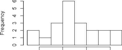
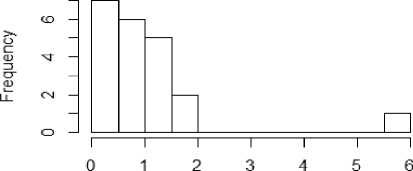
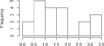
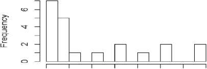
From figure 1a to 1f, the distribution of the five metrics has been displayed using histogram. The histogram with kurtosis has been repeated with eliminating of very high outlying value in 1e.

12 3 4

Entropy

Fig.1a. Histogram showing median entropy of datasets

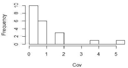
Fig.1b. Histogram showing median Coefficient of Variations of datasets

Skew

Fig.1c. Histogram showing median Skewness of datasets

Kurtosis

Fig.1e. Histogram showing median kurtosis of datasets after outlier removal

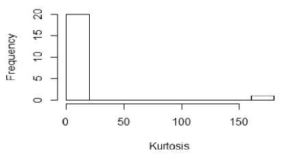
Fig.1d. Histogram showing median kurtosis of datasets

О 100 200 300 400 500 600 700

MVS

Fig.1f. Histogram showing MVS of datasets

The observations from the histograms and table 3b are as follows: -

- ‘Optdgt’ dataset, seems to be an outlier with very high value of skew, kurtosis and coefficient of variation
- ‘btissue’, ‘dow’, ‘leaf’, ‘mgc’, ‘sat’, ‘satimg’, ‘wbdc’ and ‘vehicle’ are identified as strongly correlated datasets as per the MVS score
- ‘mdlon’ has very low values for skew, kurtosis and coefficient of variation
- ‘CTG also has a relatively high coefficient of variation.

In table 4, the datasets have been coded as per the proposed scheme in table 2.

Results with Entropy:

In the below table, the results using entropy for feature elimination is presented. The 2nd to 4th columns indicate purity achieved using different feature elimination level.

Table 4a. Results with Entropy

Dataset	α = 0.1	α = 0.2	α = 25	All features
bands	0.63014	0.63014	0.63014	0.63014
btissue	0.56132	0.54726	0.5533	0.55623
CTG	0.85956	0.8142	0.77717	0.95912
Darma	0.88307	0.86721	0.86648	0.86763
Dow	0.5664	0.5599	0.55968	0.57545
Heart	0.81852	0.7963	0.81111	0.84433
hepa	0.8375	0.8375	0.8375	0.8375
Leaf	0.54309	0.55276	0.55432	0.54915
magic	0.64837	0.64837	0.64837	0.64837
mdlon	0.92267	0.91564	0.90861	0.91037
optdgt	0.65835	0.69756	0.72975	0.65516
Pen	0.74327	0.68377	0.68378	0.71778
Saeheart	0.65368	0.65368	0.65368	0.65368
satimg	0.6015	0.65212	0.64066	0.58433
satt	0.74679	0.74453	0.747	0.74611
Sonar	0.53365	0.53365	0.53365	0.53365
Veichle	0.38967	0.38142	0.38771	0.36921
waveform	0.5264	0.5268	0.5268	0.5316
wbdc	0.92267	0.91564	0.90861	0.91037
Wine	0.96067	0.95506	0.93258	0.96629
wqwhite	0.48685	0.47344	0.47349	0.47863

Table 4. Codified datasets

Dataset	SK	KT	CV	EN	MVS
Bands	LM	HM	LL	LL	SI
btissue	HH	HH	HH	LL	SC
CTG	HH	HH	HH	LM	WI
darma	HM	LM	HH	LL	WC
dow	LL	LM	LL	HM	SC
heart	LM	LM	LM	LL	SI
hepa	HM	HM	LM	LL	SI
Leaf	HH	HM	HM	LM	SC
mdlon	LL	LL	LL	HH	SI
mgc	LM	HM	LM	HH	SC
optdgt	HH	HH	HH	LL	SI
pen	LL	LM	HM	HH	WC
saehart	LM	HM	LM	LM	WI
sat	LL	LL	LL	HH	SC
satimg	HM	LL	HH	HM	SC
sonar	HM	LM	HM	LM	WI
veichle	LM	LL	HM	HM	SC
waveform	LL	LL	LL	HH	WC
wbdc	HH	HH	HM	HM	SC
wine	LL	LL	LM	LM	WC
wqwhite	HM	HH	LL	HM	WI

VI. R esults and D isucssion

This section has two parts. Initially the result using FFE has been presented for all the 5 metafeatures and 3 elimination levels. These are represented in Table 5a to Table 5e. All the tables, contain result obtained using all features in the last column.

As per the above dataset, purity at all the three levels are equivalent to purity achieved with full feature set, with the exception of the dataset ‘CTG’ and ‘Heart’, where there is a drop in purity, by more than a percentage point.

Table 4b. Results with average correlation coefficient

Datasets	α = 0.1	α = 0.2	α = 25	All features
bands	0.63014	0.63014	0.63014	0.63014
btissue	0.58642	0.57358	0.56208	0.55623
CTG	0.88315	0.88096	0.85448	0.95912
Darma	0.86201	0.86684	0.86612	0.86763
Dow	0.58095	0.56606	0.56579	0.57545
Heart	0.83704	0.82593	0.80741	0.84433
hepa	0.8375	0.8375	0.8375	0.8375
Leaf	0.51944	0.53	0.50515	0.54915
magic	0.64837	0.64837	0.64837	0.64837
mdlon	0.91037	0.91037	0.90861	0.91037
optdgt	0.65111	0.71644	0.71735	0.65516
Pen	0.71241	0.68018	0.68046	0.71778
Saeheart	0.65368	0.65368	0.65368	0.65368
satimg	0.61026	0.62405	0.65948	0.58433
satt	0.74547	0.74611	0.74566	0.74611
Sonar	0.54327	0.53365	0.53365	0.53365
Veichle	0.37194	0.3885	0.38014	0.36921
waveform	0.5278	0.531	0.533	0.5316
wbdc	0.91037	0.91037	0.90861	0.91037
Wine	0.96067	0.91011	0.88213	0.96629
wqwhite	0.45767	0.45532	0.45529	0.47863

With average correlation coefficient too, the reduction in purity is very marginal for all the three levels, so it can be said, they produce equivalent results. In fact, for datasets with high MVS, the reduced feature subsets seem to give a marginally better result on average. Only for ‘wqwhite’ and ‘CTG’ dataset, there is % drop in accuracy by more than a percentage point.

Table 4c. Results with average coefficient of variation

Datasets	α = 0.1	α = 0.2	α = 25	Full
bands	0.63014	0.63014	0.63014	0.63014
btissue	0.58642	0.57443	0.56208	0.55623
CTG	0.98159	0.98188	0.9766	0.95912
Darma	0.86388	0.86249	0.85997	0.86763
Dow	0.56626	0.55987	0.55983	0.57545
Heart	0.83333	0.82963	0.8037	0.84433
hepa	0.8375	0.8375	0.8375	0.8375
Leaf	0.54115	0.51718	0.49341	0.54915
magic	0.64837	0.64837	0.64837	0.64837
mdlon	0.91916	0.90334	0.89807	0.91037
optdgt	0.6371	0.59911	0.551	0.65516
Pen	0.70702	0.72491	0.72536	0.71778
Saeheart	0.65368	0.65368	0.65368	0.65368
satimg	0.57155	0.58788	0.58066	0.58433
satt	0.74994	0.74858	0.74837	0.74611
Sonar	0.53365	0.53365	0.55288	0.53365
Veichle	0.36725	0.37323	0.37096	0.36921
waveform	0.5284	0.5286	0.5264	0.5316
wbdc	0.91916	0.90334	0.89807	0.91037
Wine	0.93258	0.91011	0.92697	0.96629
wqwhite	0.4791	0.48244	0.48244	0.47863

With coefficient of variation, also the results are more or less similar with results obtained from all features. More than 1% performance degradation is observed in few of the datasets. The results obtained with skew as the feature elimination metric yields equivalent purity.

Table 4d. Results with average Skew

Datasets	α = 0.1	α = 0.2	α = 25	Full
bands	0.63014	0.63014	0.63014	0.63014
btissue	0.56509	0.54811	0.55	0.55623
CTG	0.87427	0.86265	0.84915	0.95912
Darma	0.85922	0.86564	0.87346	0.86763
Dow	0.56221	0.56864	0.55608	0.57545
Heart	0.77407	0.83333	0.76667	0.84433
hepa	0.8375	0.8375	0.8375	0.8375
Leaf	0.55853	0.54471	0.56118	0.54915
magic	0.64837	0.64837	0.64837	0.64837
mdlon	0.5748	0.5736	0.57745	0.91037
optdgt	0.63954	0.71443	0.72295	0.65516
Pen	0.70663	0.69376	0.66302	0.71778
Saeheart	0.65368	0.65368	0.65368	0.65368
satimg	0.63053	0.62367	0.60309	0.58433
satt	0.74561	0.74656	0.74703	0.74611
Sonar	0.53365	0.55769	0.53365	0.53365
Veichle	0.38369	0.38972	0.38652	0.36921
waveform	0.5342	0.53	0.5292	0.5316
wbdc	0.92267	0.91564	0.92794	0.91037
Wine	0.94382	0.9382	0.9044	0.96629
wqwhite	0.45788	0.46419	0.46331	0.47863

One dataset, which has a close to 30% difference in accuracy is mdlon, which is the dataset with lowest average skew.

Table 4e. Results with average kurtosis

Datasets	α = 0.1	α = 0.2	α = 25	Full
bands	0.63014	0.63014	0.63014	0.63014
btissue	0.55849	0.54717	0.5566	0.55623
CTG	0.96195	0.86769	0.85884	0.95912
Darma	0.8676	0.87793	0.87542	0.86763
Dow	0.57709	0.5804	0.5804	0.57545
Heart	0.77037	0.84444	0.84815	0.84433
hepa	0.8375	0.8375	0.8375	0.8375
Leaf	0.55118	0.55882	0.55206	0.54915
magic	0.64837	0.64837	0.64837	0.64837
mdlon	0.5628	0.54985	0.5502	0.91037
optdgt	0.65187	0.70918	0.72925	0.65516
Pen	0.69376	0.69333	0.69504	0.71778
Saeheart	0.65368	0.65368	0.65368	0.65368
satimg	0.62744	0.59537	0.58293	0.58433
satt	0.74927	0.74656	0.74744	0.74611
Sonar	0.53365	0.53365	0.53365	0.53365
Veichle	0.38771	0.38995	0.38002	0.36921
waveform	0.5186	0.5142	0.5152	0.5316
wbdc	0.92267	0.91564	0.91564	0.91037
Wine	0.96067	0.9606	0.9438	0.96629
wqwhite	0.48979	0.48032	0.47997	0.47863

One dataset, which has a close to 30% difference in accuracy, is mdlon, which is the dataset with lowest average skew. The five methods are compared in the below figure, the red line indicates purity achieved by using all the features

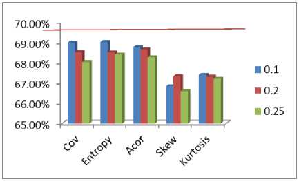
Fig.2. Comparing performance of different feature elimination strategies.

At a summary level, methods based on Coefficient of variation and Entropy is closest to purity achieved with all features. In table 5, a paired t-test has been performed between results with all features and that obtained with the 15 different feature subsets. It can be seen, for none of the 15 settings the Null hypothesis can be rejected, at 99% significance level. Hence the feature elimination strategies do not result in any statistically significant performance degradation, which was indeed one of the objectives of the study. Entropy followed by average correlation has the highest ‘p’ values for hypothesis testing. The t-statistics and p-values have been listed in table 5.

Table 5. Statistical Significance

Metric	α = 0.1	α = 0.2	α = 0.25
Cov	t = 0.6197 p-value = 0.5425	t = 1.4702 p-value = 0.1571	t = 1.8483 p-value = 0.0794
Acor	t = 0.8931 p-value = 0.3824	t = 0.7817 p-value = 0.4436	t = 1.0477 p-value = 0.3073
Entropy	t = 0.2678 p-value = 0.7916	t = 0.7698 p-value = 0.4504	t = 0.7418 p-value = 0.4668
Skew	t = 1.3917 p-value = 0.1793	t = 1.0684 p-value = 0.2981	t = 1.4722 p-value = 0.1565
Kurtosis	t = 1.0308 p-value = 0.3149	t = 1.0335 p-value = 0.3137	t = 1.0761 p-value = 0.2947

The result is illustrated, further with each individual dataset. An improvement in purity is indicated by ‘W’, a tie is indicated by ‘D’ and a loss is indicated by ‘L’. The cases where, in majority equivalent or better results are obtained are marked in bold.

From table 6, it can be observed that -

• Entropy and Kurtosis has given better or equal

result at 71.42% cases at 10% elimination level.

• Using covariance and average correlation

coefficient the same ratio is 57.14%, at 25% level,

• metrics which gives equivalent or better results in more than 50% case are Average Correlation, Skew and Kurtosis respectively across all the three levels

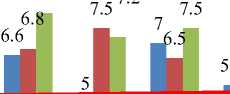
Average ranks of each of the methods are computed and compared in Figure 3.

Table 6. W-D-L by mete features

Metric	α = 0.1	α = 0.2	α = 25
Cov	W - 9, D - 3 , L - 9	W - 7, D - 3 , L - 11	W - 7, D - 3 , L - 11
Acor	W- 6, D- 6, L - 9	W- 5, D- 6, L - 10	W- 5, D- 6, L - 10
Entropy	W- 10, D- 5, L - 6	W- 6, D- 5, L - 10	W- 5, D- 5, L - 11
Skew	W - 5, D - 5 , L - 11	W - 6, D - 4, L - 11	W- 7, D - 5, L - 9
Kurtosis	W - 10, D - 5 , L - 6	W - 8, D - 5, L - 8	W - 8, D - 5, L - 8

9 8.4

8 72

6.16.3

1 α = 0.1

■ α = 0.2
■ α = 25

Cov Acor Entropy Skew Kurtosis

Fig.3. Comparing average rank of different feature elimination strategies.

The red line indicates rank achieved with all features. Kurtosis and Entropy achieves the best ranks as per the analysis.

In the table below, there is one column corresponding to each metrics and the encoded values as shown in table 4 are used. The last column indicates which of the feature elimination strategies give an equivalent or better result in average over the performance achieved with full feature set. The background color of 6th column is colored in green if FEG, correctly identifies the meta feature, Amber if fails to identify and no color if FEG can’t come to a decision and FEE needs to be applied.

Table 7. Meta feature selection strategy

Dataset	SK	KT	CV	EN	MVS	Better or Equivalent
Bands	LM	HM	LL	LL	SI	All
btissue	HH	HH	HH	LL	SC	CV, AC
CTG	HH	HH	HH	LM	WI	CV
darma	HM	LM	HH	LL	WC	EN
dow	LL	LM	LL	HM	SC	KT, AC
heart	LM	LM	LM	LL	SI	None
hepa	HM	HM	LM	LL	SI	ALL
Leaf	HH	HM	HM	LM	SC	SK , KT
mdlon	LL	LL	LL	HH	SI	EN
mgc	LM	HM	LM	HH	SC	All
optdgt	HH	HH	HH	LL	SI	ENT, ACOR, SK, KT
pen	LL	LM	HM	HH	WC	CV
saehart	LM	HM	LM	LM	WI	All
sat	LL	LL	LL	HH	SC	CV, KT, SK
satimg	HM	LL	HH	HM	SC	AC, EN, SK, KT
sonar	HM	LM	HM	LM	WI	SK, CV
veichle	LM	LL	HM	HM	SC	ALL
waveform	LL	LL	LL	HH	WC	None
wbdc	HH	HH	HM	HM	SC	SK,KT, ENT
wine	LL	LL	LM	LM	WC	None
wqwhite	HM	HH	LL	HM	WI	KT,COV

The below is the result of applying FEG strategy

• In 16 of the datasets has at least one measure as ‘HH’ or ‘SC’ in case of MVS metric. These 16 datasets have been color coded and among them in 12 of them, this is seen to be good strategy i.e. a 75% success rate.
• In 3 of the datasets there is a presence of ‘HM’ or ‘WC’, and in all three of them strategy suggested by FEG, gives correct result.
• For the rest 2 datasets, FEE needs to be applied.

VII. C onclusion

Список литературы An univariate feature elimination strategy for clustering based on metafeatures

H. Liu, and Y. Lei, "Toward integrating feature selection algorithms for classification and clustering." IEEE Transactions on Knowledge and Data Engineering, Vol.17, No.4, pp.491-502, 2005.
I. Guyon, and A. Elisseeff. "An introduction to variable and feature selection." The Journal of Machine Learning Research, Vol.3, pp.1157-1182, 2003.
Y. Saeys, I. Iñaki, and P. Larrañaga. "A review of feature selection techniques in bioinformatics." Bioinformatics, Vol.23, No.19, pp.2507-2517, 2007.
S. Alelyani, T. Jiliang, and H. Liu. "Feature selection for clustering: A review." Data Clustering: Algorithms and Applications, 2013.
Hall, Mark A. Correlation-based feature selection for machine learning. ((Doctoral dissertation) The University of Waikato, 1999.
H. Peng, F. Long, and C. Ding. "Feature selection based on mutual information criteria of max-dependency, max-relevance, and min-redundancy",IEEE Transactions on Pattern Analysis and Machine Intelligence,Vol.27, no.8, pp.1226-1238, 2005.
Estévez, Pablo A., M. Tesmer, Claudio A. Perez, and Jacek M. Zurada. "Normalized mutual information feature selection", IEEE Transactions onNeural Networks, Vol.20, no.2, pp.189-201, 2009.
T. Ignac, N. A. Sakhanenko, A. Skupin, and David J. Galas. "New methods for finding associations in large data sets: generalizing the maximal information coefficient (MIC)." In Proc. of the 9th International Workshop on Computational Systems Biology (WCSB2012), pp. 39-42. 2012.
A. Hassan, M. Shariff and N. Baksh, Awaluddin Mohd Shaharoun, and Hishamuddin Jamaluddin. "Improved SPC chart pattern recognition using statistical features." International Journal of Production Research 41, no. 7, pp.1587-1603, 2003.
S. Fong, Dept. of Comput. & Inf. Sci., Univ. of Macau, Taipa, China ; Liang, J. ; Wong, R. ; Ghanavati, M. “A novel feature selection by clustering coefficients of variations”, Digital Information Management (ICDIM) pp 205 -213. 2015.
S.Goswami and A.Chakrabarti,"Feature Selection: A Practitioner View", Internation Journaly of Computer Science and Internet Technology, vol.6, no.11, pp.66-77, 2014.
Microsft Technet SQL Server 2012, Retrieved from https://technet.microsoft.com/enus/library/ms175382%28v=sql.110%29.aspx
G. T. Wang et al., ” A feature subset selection algorithm automaticrecommendation method” , Journal of Artificial Intelligence Research, Vol. 47, pp. 1-34, 2013.
S.Goswami, A. Chakrabarti andB. Chakraborty, “Correlation Structure of Data Set for Efficient Pattern Classification”, In Proceedings of the 2nd International Conference onCybernetics (CYBCONF), pp 24-29, IEEE 2015.
X. He, C. Deng, and N. Partha. "Laplacian score for feature selection." In Proceediing of Advances in neural information processing systems . Vol. 186. pp 507-504, 2005.
Z. Zhao and H. Liu. "Spectral feature selection for supervised and unsupervised learning." In Proceedings of the 24th international conference on Machine learning, pp. 1151-1157. ACM, 2007.
S. Bandyopadhyay, T. Bhadra, P. Mitra, and U. Maulik, "Integration of dense subgraph finding with feature clustering for unsupervised feature selection." Pattern Recognition Letters, Vol.40, 2014,pp104-112.
S.Goswami, and A. Chakrabarti. "Quartile Clustering: A quartile based technique for Generating Meaningful Clusters." Journal of Computing , 2012, pp 48-57.
K. Bache & M. Lichman, UCI Machine Learning Repository [http://archive.ics.uci.edu/ml]. Irvine, CA: University of California, School of Information and Computer Science, 2013.
J. Alcalá-Fdez, A. Fernandez, J. Luengo, J. Derrac, S. García, L. Sánchez, F. Herrera. KEEL Data-Mining Software Tool: Data Set Repository, Integration of Algorithms and Experimental Analysis Framework. Journal of Multiple-Valued Logic and Soft Computing 17:2-3 (2011) 255-287.
R Core Team (2013). R: A language and environment for statistical computing. R Foundation for Statistical Computing, Vienna, Austria. ISBN 3-900051-07-0, URL: http://www.R-project.org/.
Patrick E. Meyer (2012). infotheo: Information-Theoretic Measures. R package version 1.1.1. http://CRAN.R-project.org/package=infotheo.
W. Revelle (2013) psych: Procedures for Personality and Psychological Research, Northwestern University, Evanston, Illinois, USA, http://CRAN.R-project.org/package=psych Version = 1.3.2.
S.Goswami, A.K.Das, A.Chakrabarti and B.Chakraborty, “A feature cluster taxonomy based feature selection technique”, Expert Systems with Applications, Elsevier, Vol.79, pp.76-89, 2017.
S. Goswami, A. K. Das, A. Chakrabarti and B. Chakraborty,“AGraph-Theoretic Approach for Visualization of Data Set Feature Association”, Advanced Computing and Systems for Security, Springer, pp.109-124.
L.Dey and S. Chakraborty, “Canonical PSO Based K-Means Clustering Approach for Real Datasets”, ISRN Software Engineering Journal, Hindawi, Vol.14, 2014.
S.Chakraborty and N.K.Nagwani, “Performance Evaluation of Incremental K-means Clustering Algorithm”, IFRSA International Journal of Data Warehousing & Mining, Vol.1, No.1, pp.54-59, 2011.
S.Chakraborty and N.K.Nagwani, “Analysis and study of Incremental DBSCAN clustering algorithm”, International Journal of Enterprise Computing and Business Systems, Vol.1, No.1, pp.54-59, 2011.
S. Goswami, A. Chakrabarti and B. Chakraborty, “A Proposal for Recommendation of Feature Selection Algorithm based on Data Set Characteristics”, Journal of Universal Computer Science, Vol.22, No.6, pp. 760-781, 2016.
S. Chattopadhyay, S. Mishra and S. Goswami, “ Feature selection using differential evolution with binary mutation scheme”, International Conference on Microelectronics, Computing and Communications (MicroCom), IEEE, pp.1-6, 2016.

Еще

Статья научная

An univariate feature elimination strategy for clustering based on metafeatures

Текст научной статьи An univariate feature elimination strategy for clustering based on metafeatures

II. M etrics U sed for F eature E limination

III. R elated W ork

IV. P roposed M ethod

V. M ethods and M aterials

VI. R esults and D isucssion

VII. C onclusion

Список литературы An univariate feature elimination strategy for clustering based on metafeatures