Analogue Wavelet Transform Based the Solution of the Parabolic Equation

Published Online November 2012 in MECS

filters to be constructed for stationary and non-stationary signals [2], [3]. One of the main advantages of wavelets is that they offer a simultaneous localization in time and frequency domain whereas the standard Fourier transform is only localized in Frequency domain. Wavelets have the great advantage of being able to separate the fine details in a signal. Very small wavelets can be used to isolate very fine details in a signal, while very large wavelets can identify coarse details [1].

In general the any order derivative of the Gaussian function can be employed as a mother wavelet. On the other hand since the Gaussian function is a low frequency signal, it is not suitable to be a mother wavelet, and the mother is usually a high frequency signal [4]. The hyperbolic secant/hyperbolic tangent differential operator family can be useful when we need to process highly non-band limited signals, but where we do not need all of the power of the wavelets and/or where we wish to retain the ability to process functions locally (using a fundamentally local approximation). Such operators can be used:

•

•

To calculate rough, but wide-ranging, frequency spectrum values of unknown signals.

To represent high frequency signals approximately using only (relatively) slow integrations to correct the integration coefficients [5].

One of the fundamental questions of applied harmonic analysis is to obtain density conditions on the sequences required to discretize a continuous integral transform in a way that the resulting discretization is a frame in a certain Hilbert space. This question was sharply solved for the frames in the Bergmann-Fock [6], [7], [8] and in the Bergamann space [9]. However, in the case of the Wavelet and Gabor transforms, very little is known and only a few very special windows and analyzing wavelets are understood [10]. The short time Fourier (Gabor) transform with respect to a Gaussian window can be written in terms of the Bargmann

is the reason geometry of sampling the

why everything is known about the sequences that generate frames by Gabor transform with Gaussian

g (t) = e windows

■ nt ²

. A part from this example, the

only cases where a description is known of the lattice sequences that generate frames are the hyperbolic

. g(t) = (cosh at)

secant

[11] and the characteristics

function of an interval[12], which turned out to be the nontrivial problem. There is also a necessary condition for Gabor frames due to Ramanathan and Steger [13].

One of the reasons wavelets have found so many uses and applications is that they are especially attractive from the computational point of view. Computational efficiency of wavelets lies in the fact that wavelet coefficients in wavelet expansions for functions in V L ² ( R d ) к

⁰ (resolution subspace in may be computed using matrix iteration, rather than by a direct computation of inner products: the latter would involve integration over R , and hence be computationally inefficient, if feasible at all. The deeper reason for why we can compute wavelet coefficients using matrix

iteration is an important filtering method from involving digital filters, sampling. In this setting

connection to the subband signal/image processing down-sampling and up- filters may be realized as

functions m ⁰ on a d-torus, e.g., quadrature mirror filters [14].

The wavelet transform of a signal g ( t ) is defined as

+to w (a, b) = Jg (t )^ *

-to

t - b А dt

a ) a

(the asterisk means complex conjugation)

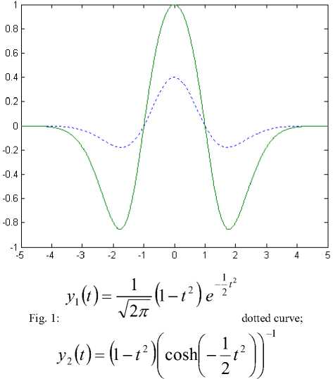
V ⁽ ^ =

top e2

e

2 л

- 5 ²

,^- i ® o 5 e 2

and the magnitude norm is used

+x

г I t - b А dt

J И---

L I a

-to

— = e a

.

curve;

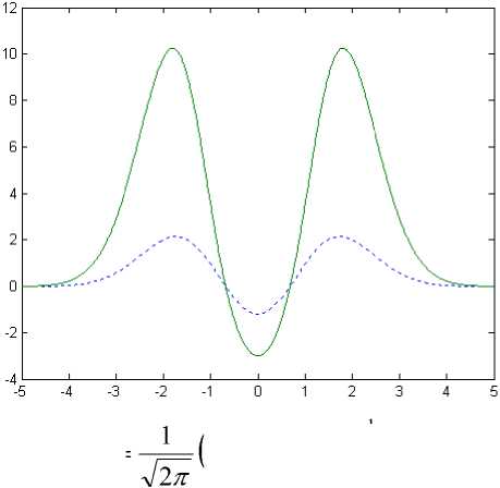
( t ⁴ + 6 t ² - з ) e

Fig. 2:

dotted

A-1

- ¹ 1 ² 2

Eqn.(1) is a derivative of the diffusively initial function [15]

n  +ro w (a, b) = an — Jg (t )^ 0 5bn _J„

t - b А dt

a ) a

smooth

The wavelet transform is also a solution of the partial differential equation [16]

. a a?

d

- - -

da

эА ito0 5b)w(a,b) = 0

The initial value is ^{w (0, b} )   g ^{( b} )

У i(t ) =

In [17] the wavelet –image is written as a sum of the real part and imaginary parts

w ( a , b ) = u ( a , b ) + v ( a , b )

y2 (t)=(t4 + 612 - з) coshl

2 X \ '

—

1t22

In this representation Eqn.(3) will be converted to the following system of partial differential equations:

8 u _  82 u

8 a      8 b ²     0 8b ’

8 v    82 v

— = a—- - ro₀ — .

8a    8b 2

h a , b ( t ) =

11 t — a । —

1     21 b J

(7 b )

and a and b represents the translation and scale of the windowed function ^{a , b ,} respectively. The term

The initial values for the real valued signals are u (0, b) = g(b), v(a, b) = 0                  (6)

^a in Eqn.(7b) is given for energy normalization at different scales [18]. Fig.3 shows respectively the real and imaginary parts represented by:

r ^{( t} ) =

The complex Morlet wavelet is given by:

	( t — a ) cos to 0 11
W a , b ( t ) =	1 b ( t — a 1	h a , b ( t )                    (7 a )
	+ sin < n 011
	L        l ь JJ

Where

and

i(t) =

2n

cos ( 2 n t ) ( 1 — t ² )

— ¹ 1 ²

e

(8a)

2n

sin ( 2 n t ) ( 1 — t ² )

— ¹ 1 ²

e

(8b)

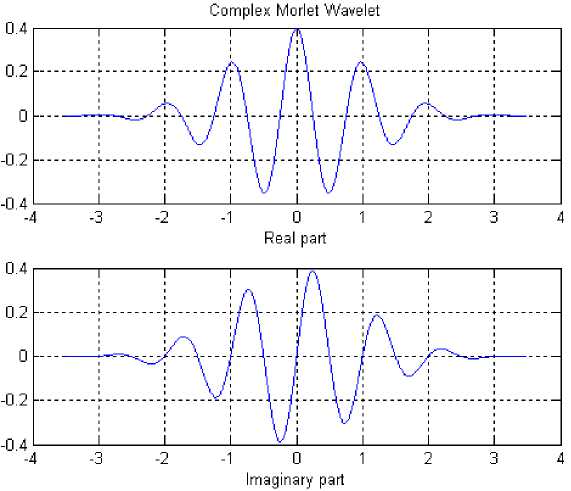
Fig. 3: Complex Morlet Wavelet

The present paper has the following sections: section two provides the solution of parabolic Equation with PDETool, section three deals with the analysis of the PDE solution using Fast Fourier Transform (FFT), and we will wind with the conclusion.

II. Solving Parabolic Equation with PDETool

Wavelets and their application for the solution of partial differential equations in physics were discussed in [19]. In this paper, we have solved the parabolic equation using PDETool. We have considered the parabolic equation

, 8 u

d--V( c V u ) + au = f 81

f = 0

If       then we say that the equation (9) is homogeneous.

In our study we have used the following PDE coefficients;

a (t) = t3 c(t) = t  d (t) = e—t f(t) = sin t

;                            ;                                    ;

where

c ( t )

is the time varying coefficient of conductivity

d ( t ) is the time varying coefficient of diffusivity           coefficients c ( t ), a ( t ), f ( t ) andd ( t ) as well as the

PDE solution to Matlab workspace.

The solution u of the equation is represented in Fig.4

and Fig.5. We have then exported the time varying PDE

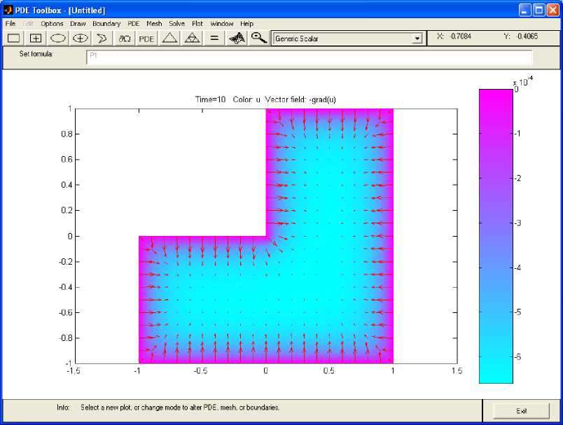
Fig. 4: PDE Solution with Arrow Plot

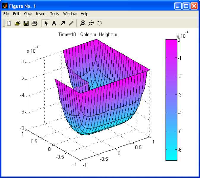
Fig. 5: PDE Solution with Height Plot

The solution u was imported from Matlab workspace to signal processing tool with the sampling frequency of 8192Hz. This tool has three main components: signal section view, filter section view and edit as well as spectra section. These are used to visualize waveforms and spectra of several signals and make a qualified filter design. Therefore, characteristic properties and desired parameters of the solution have been estimated. In order to use the PDE solution under these processes the solution was imported as a real array of consisting of 11 column index vectors each having 557 data points.

There are two ways from which one can generate analogue wavelet transform from PDE solution:

• 1.    Either one can directly use the PDE solution and apply a properly designed band pass filter as per Fig.8. and Fig.9. or

• 2.    Alternatively one can compute the Fast Fourier Transform of the PDE solution and apply the same filter.

Let ^{5 (} t ) = ^{[ 5} 1 ⁽ t )    ⁵ 2 ⁽ t )   .   .   . s n ⁽ t ^{) ]}

be the sampling vector signal

Let x ⁽ t ) = ^[ x 1 ⁽ t )    x 2 ⁽ t )   .   .   .    x n ⁽ t ) ]

be the sampled vector signal

Let y ( t ) =^[ y i ( t )    y 2 ( t )   ■   ■   ■    У п ( t ) ^]

be the response of the band pass filter x 1 (t) = u 11 s 1 (t) + u 21 s 2 (t) +... + un 1 sn (t)

= EX S k ( t )

i = k = 1

x ₂ ( t ) = u ₁₂ s 1 ( t ) + u ₂₂ s ₂ ( t ) + ... + u n ₂ s_n ( t )

= E u / 2 x k ⁽ t )

i = k = 1

x m ⁽ t ) = u 1 m s 1 ⁽ t ) ⁺ u 2 m s 2 ⁽ t ) ⁺ ... ⁺ u nm s n ⁽ t )

n

= E u m s k ⁽ t )

i = k = 1

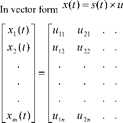
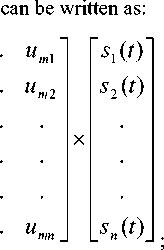
be m x n pde solution matrix where m = 11 and n = 557

^{m x 1 1}

This data matrix is a real matrix, ^{u G R}    ,

associated with ^{m x n} points of the PDE solution. In this section we attempt to express the sampled vector

P xm

= |xm (t)Г =

n

E u m s k ⁽ t )

i = k = 1

signal x ( t )

in terms of sampling vector signal

s(t)

as

Total power of the sampled PDE solution is:

well as data matrix u representing the PDE solution.

Let f ( t ) be the impulse response of the band pass				Power of the sampled PDE solution
filter				From the definition of power the power associated to
				sampled PDE solution is given by:
	u 11      u 12     .	.     u 1 n
						2
	u 21     u 22     .	.    . u 2 n		P x, =1 x . < ‘ )| 2 =	EE u - 1 s k ( t )
Letu =	.                    .              .	..   .	(10)		= k = 1
	.                    .              .	..   .				2
	.                    .              .	..   .		P x 2 = | x 2 ( t )2 =	E u - '2 s k ( t )
	U 1 U 3 m 1       m 2     .	. u mn _			i = k = 1

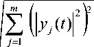
P x       P^ + ( P x 2 ^{) 2} + .... + ( P x m ^{) 2}

m 2

=J Z⁽i x j ( t ) )

V j = 1

m z j = 1

n

Z u ij s k ⁽ t )

i = k = 1

Energy of the sampled PDE solution

+to

+to

n

E x 1

= ji x i ( t )² d = j z u n s k ( t )

-to

-to

V

i = k = 1

² I dt

+»

+to

n

E x 2

= j | x 2 ⁽ t )| dt = j Z u i 2 s k ⁽ t ) ^dt

-to

-to

i = k = 1

+to

+to

n

E xm

= j x m ⁽ t )| ^dt = j Z u m s k ⁽ t)  ^dt

-to

-to

i = k = 1

Total energy of the sampled PDE solution is:

Ex =V(Ex )2 +(Ex )2 +.... + (Ex)

x            x1           x2

From Eqn. (11) we obtain:

E x

m 7^to

Z j ^j = 1 V -to

m <№I

Z jl x1( t)dt j=i V-to

n

Z u ij S k ( t )

i = k = 1

² I ² dt

By definition the response of the band pass filter is

given by the convolution of the impulse response

f ( t )

of the band pass filter with the sampled vector

Hence we get:

+to

У ( t ) = f ( t ) * x ( t ) = j x ( t ) f ( t - т ) d T

-to .

Apply the above definition to each column, we get:

+to

У1(t) = x1(t) * f (t) = j x1(t) f (t- T)dT to

+?7

= j l Z u i 1 s k ⁽ t ) I f ⁽ t ^{- т} ) ^{d T}

-toV i=k =1

"

= Z ui 1 j sk(t) f(t- т)dT i=k=1

+to

У 2 (t ) = x 2 (t ) * f (t ) = j x 2 (t )f (t - T ) d T to

7Г

= j l Z u i 2 s k ⁽ t ) I ^{f (} t - ^T ) ^{d T}

-toV i=k =1

"+to

= Z ui2 j sk (t)f(t - T)dT i=k=1

+to

Ут (t) = xm (t) * f (t) = j xm (t)f (t - T)dT to

⁺?7 "

= j l Z umsk ⁽ t ) I f ⁽ t ^{- T} ) ^{d T}

-toVi=k =1

"+to

= Z uim j sk (t)f(t - T)dT i=k =1

The filtered PDE solution y ( t )

is shown in Fig. 10.

The filtered PDE solution is a modulated signal. Hence we have generated analog continuous wavelet transform from PDE solution.

The Matlab signal processing tool shows that the modulated signal generated out of the PDE solution is a real signal. Its expression can be derived from the equation of complex mother Morlet equation given in Eqn. (7a) by equating the imaginary part to zero. Hence we get

y i ( t ) = W a i , b i ( t ) = h a i , bi ( t )cos to o I t—a i- I (13) V b i  7

We can therefore see that the filter effect has generated a wavelet transform that is proportional to the windowed function.

signal x ⁽ t ) = [ x 1 ⁽ t )    x 2 ⁽ t )   . .   .    x " ⁽ t ^{) ]} .

Power of the filtered sampled PDE solution

P =1 y .< t )l2

Py 2 =1У 2< t f

Py. = |Ут (t)|2

n        '^M

Z U 1J sk(t) f(t — T) dT i = k=1    —m

n         '^M

Z ui 2 J sk (t)f(t - т) dT i = k=1    —m

n      +m

Z Um J sk (t)f(t — T)dT i=k =1    —m

Total Power of the filtered sampled PDE solution can be computed considering it as a vector with components.

22   2

У   \\yj ⁺ \ yy 2/   •" ⁺ \ ¹ y.)

Py =

m z j = 1

n     ^+M

Z U m J sk (t)f(t — T)dT

I = k = 1     —^

2)2(14)

J

Energy of the filtered sampled PDE solution

+^

Ey_ = J|y,( t )|2 dt

—M

+»

-J

—M

n     +M

Z u11J xk (t) f(t—т) dT i=k=1    —m

dt

+m

Ey2 = Ji y 2( t )2 dt

— M

+ M n     +M

= J Z Ui2 J Xk (t)f (t — T)dT

— M i = ^k = ¹     —M

dt

+M

Ey. = Jiy. (t )2 dt

— M

+ M

n

+ M

= J Z Uim J xk (t)f(t — T)dT dt

—

M

i = k = 1

—

M

Total energy of the filtered sampled PDE solution can be computed considering that this energy is a vector. Then the magnitude of that energy is given by the following formula:

Ey =V(Ey )2 +(Ey )2 + ••• + (Ey )2

y          y ₁            y ₂                  y _m

From Eqn. (14) we get:

Ey =

:Z J j=1

m <⁺M.

Z JIyj(t)| dt j =1 V—M          J

n    ^+M

Zu-1J xk(t) f(t—t )dT i=k=1   —m

2   )2

dt

J

The sampled PDE solution is shown in Fig.6. It was computed using music method of power computation. The power spectral density (PSD) of the PDE solution is shown in Fig. 7 with minimum frequency equal to half of the sampling frequency.

A stable band pass filter has been designed to analyze in this frequency range the PDE solution. Fig.8 indicates the pole–zero plot of the filter. Magnitude, phase response, step response, group phase delay and other properties of the same filter are shown in Fig.9.

The filtering process has eliminated noise successfully as indicated by power spectral densities (PSDs) of pre-filtering and post-filtering. The filtered signal is a modulated signal shown in Fig.10. The PSD of the filtered PDE solution is shown in Fig.11.

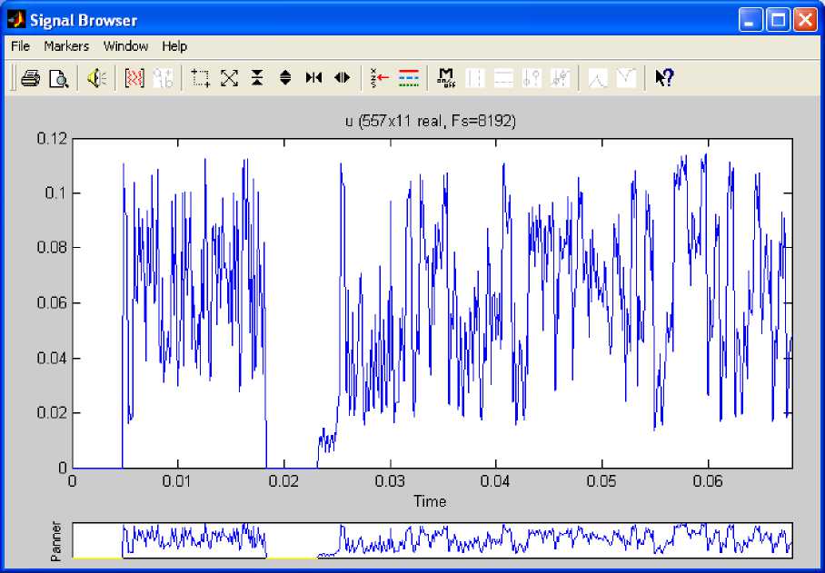
Fig. 6: Sampled PDE Solution for Column Index Vector 2

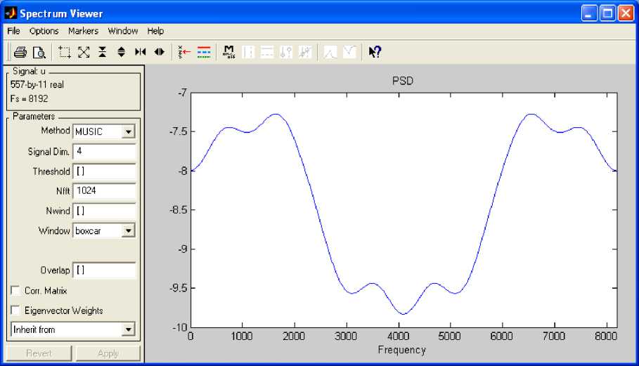
Fig. 7: PSD of Sampled PDE Solution

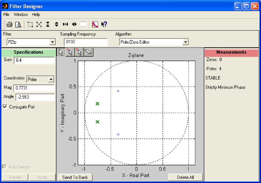
Fig. 8: Filter Pole-Zero Plot

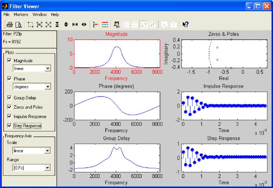
Fig. 9: Filter Characteristics

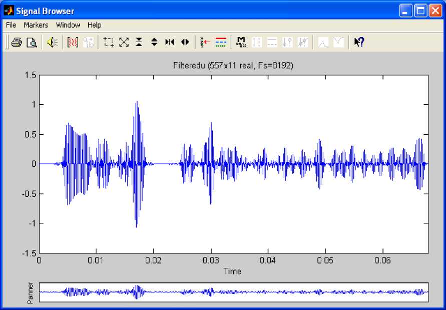
Fig. 10: Filtered PDE Solution for Column Index Vector 2

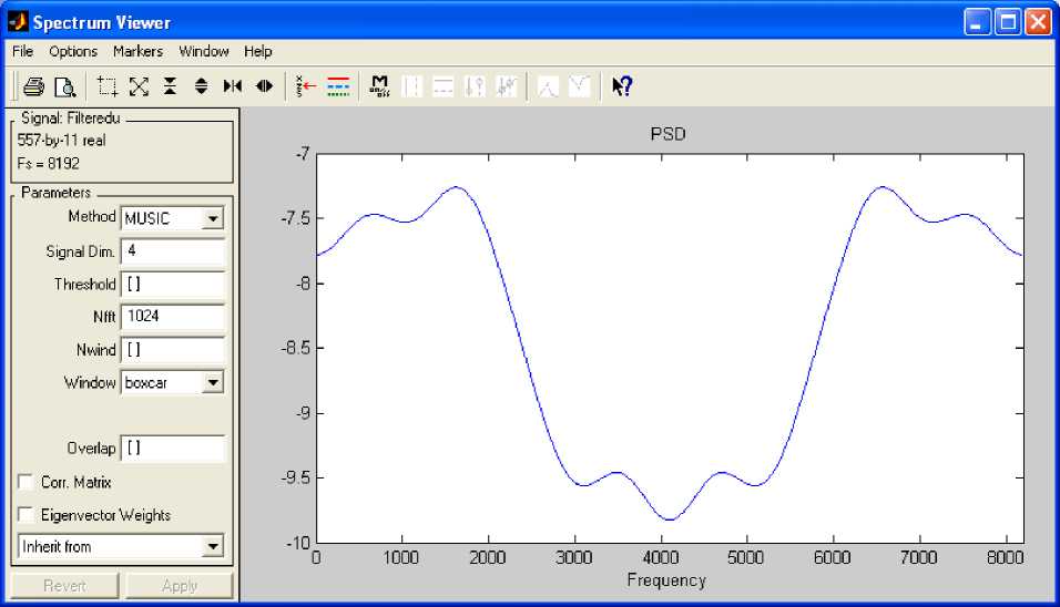
Fig. 11: PSD of Filtered PDE Solution

• III.    Spectrum Analysis with the FFT

Let us now explore the frequency analysis of the PDE solution through the computation of the Fast Fourier Transform. Unlike PDE solution discussed in the previous section the computation of FFT generates points which are complex in nature. The plot of fft(u) is shown in Fig.12. The complex points of the FFT of the PDE solution are imported from Matlab workspace to Matlab signal processing tool with the same sampling frequency. Fig.13, Fig.14, Fig.15 and Fig.16 show the real the part, imaginary part, magnitude and phase angle of the Fast Fourier Transform of the PDE solution respectively.

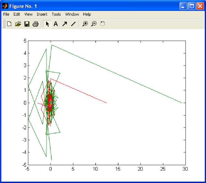
Fig. 12: FFT of PDE Solution

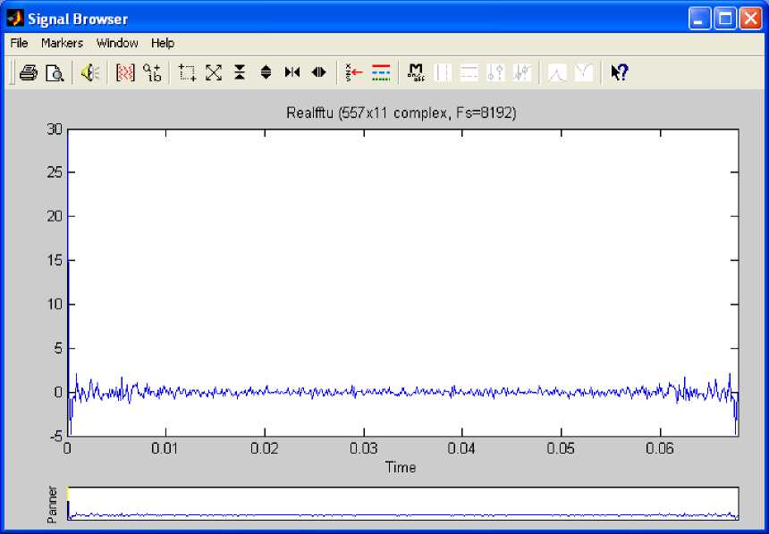
Fig. 13: Real Part of fft(u) for Column Index Vector 2

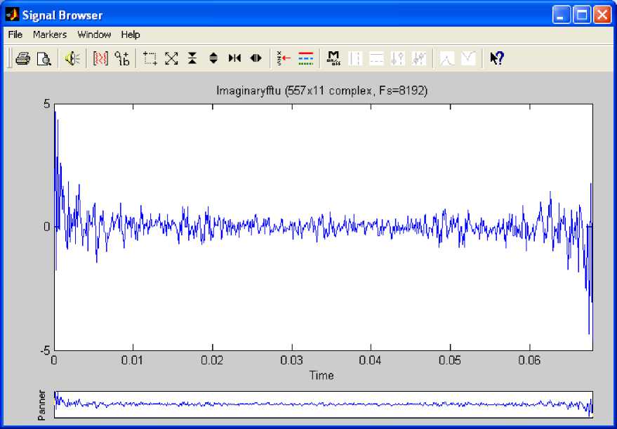
Fig. 14: Imaginary Part of fft(u) for Column Index Vector 2

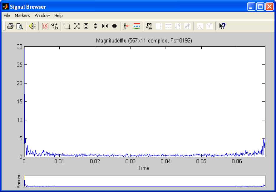
Fig. 15: Magnitude of fft(u) for Column Index Vector 2

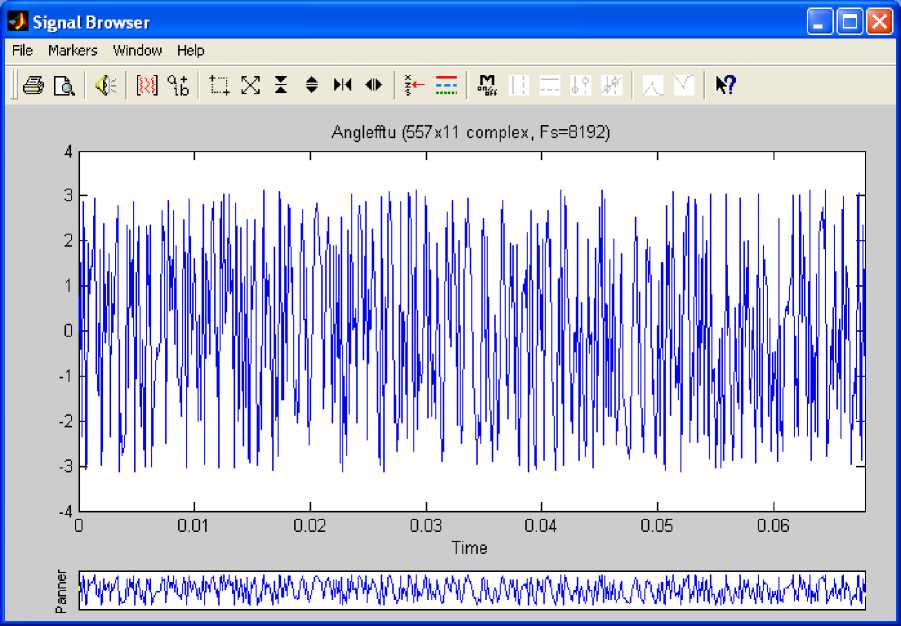
Fig. 16: Phase Angle of fft(u) for Column Index Vector 2

The FFT does not directly give you the spectrum of a signal. The FFT contains information between 0 f and s , however, we know that the sampling frequency must be at least twice the highest frequency component. Therefore, the signal’s spectrum should be entirely fs below 2 , the Nyquist frequency. Recall also that a real signal should have a transform magnitude that is symmetrical for positive and negative frequencies. So instead of having a spectrum that goes from 0 to fs , it would be more appropriate to show the spectrum from fs      fs

- - -

Let c(t)   [c 1(t)   c2(t)   .   .   .   cn (t)]   be the sampled vector signal

Let w(t) = [w1(t)  w2(t)  .  .  . wn (t)] be the response of the band pass filter

Let f ( t ) be the

impulse response of the band pass filter z11    z12

z 21     z 22

Let fft (u) = z1n

^z 2 n

The computation of the FFT allows the analysis of the PDE solution in frequency domain. It therefore provides additional information to the existing ones on the PDE solution, especially on the power spectral density. The filtered real part, imaginary part, magnitude and phase angle of the Faster Fourier Transform of the PDE solution are respectively shown in Fig.18, Fig.19, Fig.20 and Fig.21, whereas the power spectral density (PSD) of the filtered Fast Fourier Transform of the PDE solution is shown in Fig.22.

Let 5 ⁽ t ) = ^[ 5 1 ( t ) 5 2 ( t ) . . . s n ⁽ t ^{) ]} be the sampling vector signal

L z m 1

z m 2

z mn

be m x n pde solution matrix where m ¹¹ and

n = 557

.

The data matrix in Eqn.(16) is a complex matrix,

fft ( u ) e Z m ^{x n}

associated with m x n points of the FFT of PDE solution. The Matlab signal processing tool shows that the sampled PDE solution is a complex array consisting of 11 column index vectors each of 557 complex data points. In this section we attempt to express the sampled vector signal

c(t) in

terms of sampling vector signal

x(t)

as well as data

Pc 2 = C 2( t )|2

n

E z ^ s k ⁽ t )

i = k = 1

matrix

fft ( u )

representing the FFT of PDE solution.

C1 (t) = z 11 s 1 (t) + z21 s2 (t) + ... + zn 1 sn (t) n

= E zn sk (t)

i = k = 1

PCm = Cm (t )|2

n

E z m s k ⁽ t )

i = k = 1

C2 (t) = z 12s 1 (t) + z22s2 (t) + ... + zn2sn (t)

Total Power of the sampled PDE solution

n

= E ui2 sk (t)

i = k = 1

PC = V(PC?T +(PC2 )2 + .- +(PCm )2

m

=A El cj (t )l

\ j = 1

cm (t) = z 1 ms 1 (t) + z2ms2 (t) + ... + znmsn (t)

= EEzimsk (t)

i = k = 1

In vector form ^{C (} t )   s ⁽ t ) ^X fft ⁽ u ) can be written as:

C 1 ( t )"		z 11	z 12     .	.     z 1 n		" s 1 ( t )
c 2 ( t ) . .	=	z 21 . .	z 22     . .. ..	.    z 2 n .              . .              .	x	s 2( t ) . .
. C m ( t ) J		. , z m 1	.. z m 2    .	.              . . z mn _		. L s n ( t )

Power of the sampled FFT of PDE solution

Pc, = C1( t )|2

n

E z11 sk(t)

i = k = 1

;

Energy of the sampled FFT of PDE solution

+^

Ec, = ji c,( t )2 dt

-to

= j E zu sk(t)

+to

-to

n

i = k = 1

+to

EC2 = j| C 2(t )| dt

-to

+ to

n

dt

= j E zi2 sk (t) dt

-to

i = k = 1

+to

E c m = J C m ( t ) dt

—to

П      +to

= E zi-1J sk(t) f(t—т)dT i = k=1    —to

+ to

n

= J E z im s k ⁽ t )   ^dt

w 2 ⁽ t ) = ^C 2 ⁽ t ) * ^{f (} t )

-to

i = k = 1

Total energy of the sampled FFT of PDE solution is given by:

+ to

= J C2(t)f (t — T)dT to

E C =Л E C ) ² +⁽ E C 2 ) 2 + ... + ^{( E} C _ ^{) 2}

^+to< n            A

= J l E zi 2 xk ⁽ t ) I f ⁽ t ^{— т} ) ^{d T}

—to V i = ^k = 1            /

Using Eqn.(17) we obtain:

E c

m ^+to

E J Icm (t)| ^t j =1 —to

n

E i = k =1

f     ⁺to                     )

z i 2 J s k ⁽ t ) ^{f (} t ^{— T} ) ^{d T}

V     —to                     7

m f +”

E J j=1 ^—to

n

E zu sk(t) dt i=k=1

w m ⁽ t ) = c m ⁽ t ) * ^{f (} t )

+to

= J cm (t)f (t — T)dT to

By definition the response of the band pass filter is given by the convolution of the impulse

+to/ n            A

= J l E z im s k ⁽ t ) I ^{f (} t — ^T ) ^{d T}

_—to V i = k = 1            7

response

w ( t )

vector signal.

of the band pass filter with the sampled

n

= E

l zm

i = k = 1 V

+to                      ^

J s k ⁽ t ) ^{f (} t - ^T ) ^{d T}

—to                       7

^{C (} t ) = ^{[ c} 1 ⁽ t )     ^C 2 ⁽ t )   .   .   . ^C n ⁽ t ^{) ]}

Hence we get

+to w (t) = f (t) * C (t) = J c (t) f (t — т) dT

—to

Apply the definition to each column, we get:

Power of the filtered sampled FFT of PDE

solution

p w = w 1 ( t )|²

n      ^+to

E zi-1J sk(t)f(t—т)dT i = k=1    —to

^w 1 ⁽ t ) = ^C 1 ⁽ t ) * f ⁽ t )

+to

= J C 1( t) f (t — т) dT to

P . 2 = w 2 ( t )| 2

n       +to

E zi2 J xk (t)f (t — T)dT i=k =1    —to

n

_ vl E z i i x k ⁽ t ) I f ⁽ t ^{— т} ) ^{d T}

= J V i = k = 1          7

—to

^P . m = W m ( t )|²

n       +to

E z im J x k ⁽ t ) ^{f (} t — ^{T ) d T} i = k = 1      —to

Total Power of the filtered sampled FFT of PDE solution

P. = J(P.J2 + (P., )2 + ... + (P.m У

+да

Ew2 = J w2(tf dt

-да

m

E(lwm (t)| ) j =1

+да

—J

-да

n       +да

E wi2 J sk (t)f(t- т)dT i—k—1     —да

dt

J

m

E [

n    +”

E zi i J xk(t) f(t —T)dT i—k =1    —да

J

+да

Ew„ — J wm (t)Г dt

—да

+да

—J

—да

n       ^+да

E zim J sk (t) f (t — T)dT i — k—1     —да

2) dt

J

Energy of the filtered sampled FFT of PDE solution

+да

Ew. — J И(tf dt

—да

Using definition and Eqn.(19),the total energy of the filtered sampled FFT of PDE solution is given by:

+да

-J

—да

n      ^+да

E zi i J sk(t) f(t —т)dT i—k—1    —да

2 ^

dt

J

E. — V(E.1)2 +(E., )2 + ... + (Ewm )2

m ^ +да

E J Pm (t)Г dt j—1 \—да

J

m ^ +^да

E J

j ^{— 1} ^ —да

n      +да

E ui 1 J s k ⁽ t )■ f ⁽ t ^{— T} ) ^{d T} i — k — 1     —да

2   12

dt

J

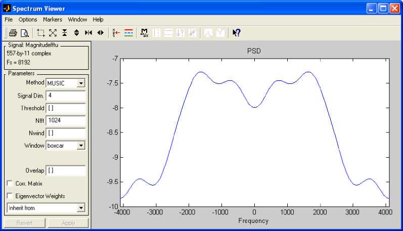
Fig. 17: PSD of fft (u)

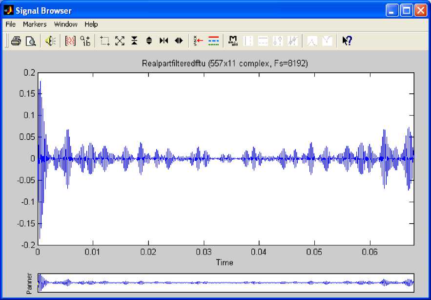
Fig. 18: Real Part of Filtered fft (u)

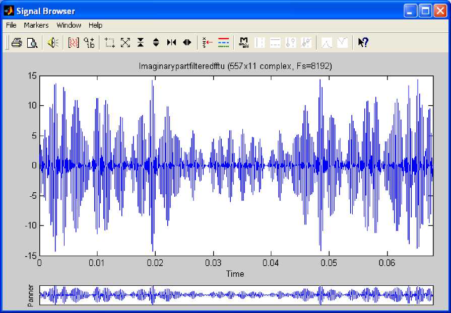
Fig. 19: Imaginary Part of Filtered fft (u)

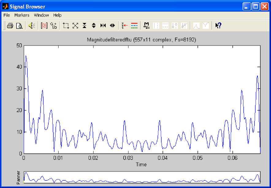
Fig. 20: Magnitude of Filtered fft (u)

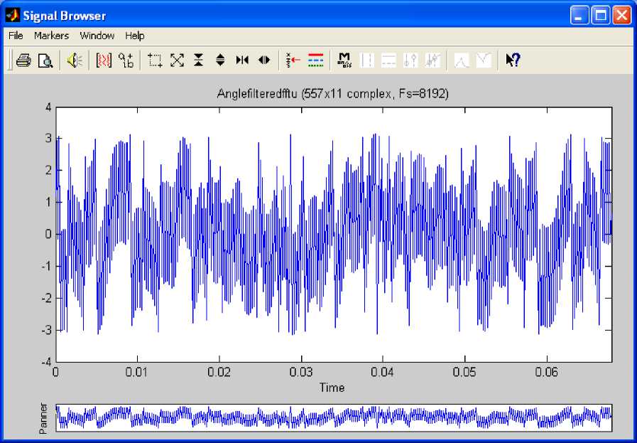
Fig. 21: Phase Angle of Filtered fft (u)

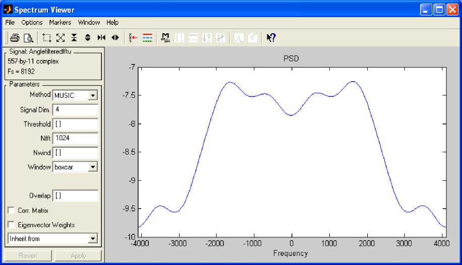
Fig .22: PSD of Filtered fft (u)

• IV.    Conclusion

In our research we have proved that the PDE solution generates analogue wavelet transform. We have imported the PDE solution from Matlab workspace to signal processing tool. We have sampled the imported PDE solution and applied the band pass filter to it. The convolution of the sampled PDE solution with the impulse response of the band pass filter has generated analogue wavelet transform. This algorithm computes the analogue wavelet transform either directly of via Fast Fourier Transform. The computation of the FFT of the PDE solution has produced complex wavelet transform. The FFT provides analysis of the PDE solution in frequency domain.