Analysis and Forecasting of the Time Series Data on Births and Deaths in Azerbaijan Using ARIMA Model

Forecasting of population data is enable understanding the future trend of socio-economic development and proper allocation of available resources. Population growth is determined by births, deaths, and migration. The predictions of birth and death are a key input to estimation of population size, but they are surrounded by significant uncertainty, leading to important differences in population predictions. These differences between predictions and actual data could compound over many years and significantly affect outcomes by the end of the projection period. The statistical accuracy of forecasts is particularly important, and the methods used to generate reliable estimates must match the observed patterns in birth and death and must perform well in terms of predicting uncertainty. Birth and death forecasts can be made (produced) using univariate or multivariate statistical time series methods, structural models or machine learning (ML) methods [1]. Global population projections have been produced by the Population Division of the Department of Economic and Social Affairs of the UN Secretariat (UNPD) since the 1950s. For many years, UNPD used a deterministic model for fertility, mortality, and migration [2]. Gusev A. et al. examined the possibility of creating and comparing short-term predictive mortality models of a region's population using CatBoost ML methods in the preCOVID (2019) and COVID period (2020). For the 2019 data, the model error is decreased as the learning period increased, but for the 2020 data, this decrease was not observed [3]. In [4] has been examined the use of the ARIMA model for forecasting of coronavirus infection and deaths in a number of regions of the Russian Federation. It was shown that the resulting forecast made it possible to fairly accurately predict the total number of infections and deaths for 7–10 days. It turned out that the model parameters are different for time series of different lengths, for different regions, in addition, the model parameters change over time. Bravo and Coelho [1] evaluated the forecasting performance of seasonal ARIMA, Holt-Winters and State Space (SS) models applied to birth and death monthly forecasting at the sub-national level. They also investigated how well the models perform in terms of predicting the uncertainty of future monthly birth and death number. The results of experiments shown that, SS models show better performance for births and seasonal ARIMA for deaths.

The ARIMA models and AR models are used for forecast the Total Fertility Rate (TFR) in Malaysia and the forecasting performance of these models is evaluated by using post sample forecasting accuracy criterion. It was found that the AR model could be the most appropriate model for forecasting the TFR in Malaysia [5]. In [6] five different forecasting models (including Mean model, Naïve model, ARIMA model, Exponential State Space model and Neural Network model) were used for predicting the infant mortality rate (IMR) in Malaysia. The results showed that the ARIMA (0,2,0) model is the best model.

• D. Lancheros-Cuestaet al. [7] tested the application of an ARIMA forecasting model to obtain future estimates for birth and death data in Colombia. The analyzed data has been sorted as national and by departments as well. Close approximations in the years of study were obtained from the general data. The actual birth and death data for 2016 for eleven departments were compared with the ARIMA results. This model was found to fit properly with the data used in this study and show reliable prediction with low percentage error. Also, the best strategy for analyzing time series is to have a large amount of specific data. When the data is generalized, errors are not considered, and if there are big errors, the model may tend to be inaccurate.

In [8] has been successfully modelled and analysed the ARIMA model under classical and the Bayesian paradigms. The analysis resulted in projections of India's IMR data for the next 5 years. Stationarity of the data set was carefully checked using ADF and KPSS tests. The likelihood-based estimates were used for the classical predictions, and corresponding modal values of parameters were used for Bayesian predictions. It turned out that the latter paradigm was found to provide more accurate and reliable results than the former.

• Y. Chen and Abdul Q. M. Khaliq [9] applied the three popular RNNs model, which are Long Short-Term-Memory (LSTM), Bidirectional Long Short-Term Memory (BI-LSTM), Gated Recurrent units (GTU) and the Lee-Carter model to mortality rate prediction in USA. The study based on the yearly-age mortality rate data from 1966-2015 of the United States. A multivariate three layers deep learning networks architecture is used for each model. According to the average performance, the Bi-LSTM gave the best average prediction results with 0.00299874/0.0066071 (MAE/RMSE). They found that every deep learning model gave a comparable performance to the Lee-Carter model.

In [10] has been used the Multiplicative Seasonal ARIMA model to predict underlying seasonal time series for COVID-19 mortality rates. The COVID 19 data, which was collected between 2020-10-04 and 2021-05-12 by the Hungarian government and the World Health Organization (WHO), has been used. Based on the Autocorrelation Function (ACF) and Partial Autocorrelation Function (PACF) plot data, the proposed ARIMA model was determined to be the best model for predicting the daily mortality rate of COVID-19 in the country.

• Y. Wang [11] applied the ARIMA and the ETS models to forecast the short-term birth rate in China in the next five years. The historical fertility rate data in China from 1964 to 2021 used in study. From the Results shown that the time series plots of these two models have similar trends. Author found that the ARIMA model was more appropriate for predicting the short-term birth rate in China. As a result, was utilized the ARIMA (0,0,1) model for prediction.

• B. A. Masha et al. [12] examined Ghana's birth rate using the Box- Jenkins technique on a monthly basis. Monthly data ranging from January, 2014 through to December 2019 was collected from Ghana Statistical Service. They discovered that the ARIMA (1, 1, 1) model had the best fit, with the lowest normalized BIC and AIC values among the tested models. This model was applied to the 12-month birth rate for the year 2020.

• L. Onambele et al. [13] used the ARIMA model, Holt method and the ML Prophet Forecasting Model (PFM) for forecasting maternal mortality rates (MMRs) for the next 15 years in Africa. MMRs and population data were extracted from all African countries’ World Bank mortality databases from 1990 to 2015. Research has shown that the projections computed by the ARIMA, PFM, and Holt methods are similar, and their confidence intervals overlap. Also, PFM outperforms traditional models like ARIMA and SARIMA. Additionally, PFM has a significantly faster training time, about ten times quicker than ARIMA. However, this study’s 25-year dataset provides a robust basis for projecting trends 15 years into the future, capitalizing on the ARIMA model’s ability to detect long-term patterns.

2.    Materials and Methods 2.1.    Dataset

Currently, Azerbaijan is among the countries facing a decline in the birth rate, on the other hand, mortality statistics are not stable. This means that the country is under serious threat in the future due to the aging of the population. In this regard, obtaining forecasts of birth and mortality can focus the attention of politicians on solving these problems. As can be seen from the above studies, the ARIMA model is widely used in the forecasting of birth and mortality time series, along with ML methods. The ARIMA model is simpler, it is fitted for the annual series and it is applicable for the annual series which does not contain any seasonal components. However, time series forecasting methods have not been tested in our country in the forecasting of birth and mortality. For the first time, the ARIMA model has been evaluated in the context of forecasting birth and mortality in Azerbaijan. The aim of this work is to build an appropriate ARIMA model for birth and mortality time series data and to make an accurate forecast of the number of births and deaths in Azerbaijan for the next eight years.

In this study, we use demographic data for Azerbaijan comprising data on live births and deaths (non-fetal deaths) broken down by years provided by Statistics Committee of the Republic of Azerbaijan. This information is obtained based on monthly statistical elaboration of birth and death statements compiled by registration Office of the Ministry of Justice. The data is located on the website of the statistical committee and the website gives the option to choose which data to download by year [14]. The required data for the study, (births and deaths data ranging from January, 1950 through to December 2022) was downloaded from the website of Statistics Committee. A database is created in Excel with all the downloaded information from the website, sorting the data by year. With this information, the necessary conditions for the model to forecast accurate predictions are determined. These data were plotted on the graphs, as shown in Fig.1. The univariate ARIMA model was applied to predict the number of births and deaths for the next years. The data analysis has been performed using Python programming languages and its Scikit Learn library.

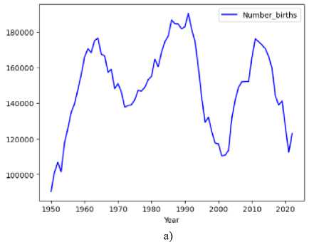
Fig. 1. Time series plot of the yearly number of births (a) and deaths (b) as on 1950 to 2022.

From the graph, it can be seen that non-positive demographic trends in the country, and there is no a stable growth rate or decline of the birth or death.

• 2.2.    ARIMA model

ARIMA is a statistical model used for analyzing and forecasting time series data. It also popularly is known as the Box-Jenkins method [15]. The ARIMA is approach providing a flexible and structured way to model time series data based on its prior observations as well as past prediction errors. ARIMA models are, the most general class of models for forecasting a time series which can be made to be “stationary” [16]. A stationary series has no trend (increase or decrease), its fluctuations around its mean value have a constant amplitude, and it moves in a consistent manner. The ARIMA forecasting equation is a regression-type equation in which the predictors consist of lags of the dependent variable or lagged forecast errors. An ARIMA model is classified as an "ARIMA (p, d, q)" model, where:

• -    p is the number of autoregressive (AR) terms, also known as the lag order.

• -    d is the minimum number of differences needed for stationarity. Also, it known as the degree of differencing. If the time series is stationary, then d = 0.

• -    and q is the size of the ’moving average’ (MA) window. q is the number of lagged forecast errors in the prediction equation.

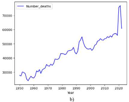
The steps (stages) of the ARIMA model building methodology are presented in Fig.2. In the analysis, the Box-Jenkins methodology followed when building an ARIMA model. This methodology consists of four steps. The first step is called identification, and the aim of this step is to make sure that the series is stationary and identifying appropriate lags for the components of the AR and MA. The Auto Correlation Function (ACF) and the Partial Auto Correlation

Function (PACF) are used to find out the appropriate values of p, d, q in the first step, and determine the best ARIMA model. The second step in the analysis is to estimate of the parameters in the model. The process of least-squares estimation is usually used for this [15].

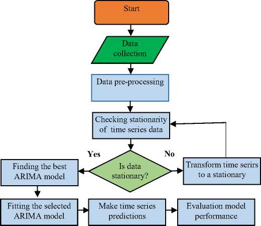
Fig. 2. The stages of the ARIMA model building methodology.

The next (third) step is diagnostic testing, which check residuals of the fitted model to determine the adequacy of the chosen ARIMA model. If the residuals are not white noise, then the first, second, and third steps are repeated again using the new values for p, d, and q [17].

Forecasting is the fourth step where the ARIMA time series models may be used to predict future values. The best ARIMA model was selected based on minimal AIC and BIC values. The Ljung-Box test was used to evaluate the stability of the model.

The performance of the models in terms of predicting the uncertainty of future births and deaths is determined by the 95% prediction intervals associated with each set of forecasts. If the deviations from the 95% prediction interval are too large, the model is considered to fail in terms of predicting the uncertainty.

The performance of the learning models is measured using the value of the MAPE and RMSE. MAPE expresses the average absolute percent difference between actual and predicted values. The RMSE measure is defined as the square root of mean square error. Lower values of these measures generally signify better model accuracy [16, 18].

3.    Results and Discussions

In this section, experiments are conducted and their results are summarized. Our target is to build an ARIMA model in Python that can predict the number of births of deaths for the next 8 years (2023-2030 years) in Azerbaijan.

• 3.1.    Forecasting the number of births data

The dataset used in our study is based on yearly births size in Azerbaijan. This data was plotted on a graph, as shown in Fig.1 (a). The births dataset is divided into training (90%) and testing (10%).

As mentioned earlier, ARIMA models usually applied on stationary time series. For this, we first check the stationarity of the time series. That is, we check that the statistical properties of our time series remaining approximately the same over time. There are different ways of checking whether the time series is stationary. For investigation of the stationarity of the time series, Augmented Dickey-Fuller (ADF) (and Kwiatkowski-Philip-Schmidt-Shin (KPSS)) test was applied for the training series in this study. The null hypothesis of ADF test is that the data are non-stationary. Therefore, large p-values indicate the data non-stationarity while small p-values imply the reverse. The results of applying KPSS, ADF tests are shown in Table 1.

Table 1. p-values for ADF and KPSS for training series.

Test	ADF	KPSS
p-value	0.0003	0.1

As seen in Table 1, the p-value of KPSS is 0.1 which is greater than 0.05, while the p-value of ADF test is less than 0.05 (p-value=0.0003), it indicates, that the birth data is stationary, so there is no need for differencing. Note that, differencing is required for stationarity of time series when the p-value is greater than 0.05.

The ACF and PACF were used to classify the ARIMA (p, d, q) model. The ACF and PACF correlograms of births data with the 95% confidence interval were shown in Fig.3.

(a)

(b)

Fig. 3. ACF (a) and PACF (b) plot for births time series data.

The best suitable ARIMA model for birth time series was selected based on minimal AIC and BİC values. The Ljung–Box test was used to evaluate the stability of the model. The p value of Ljung–Box test of the ARIMA models (except for the t ARIMA (1,0,1) model) is greater than 0.05. It indicates that the residual of selected model conforms to the characteristics of white noise sequence, and model was suitable for forecasting. Using the cross-validation method, data 90% were selected as the training set and data 10% were selected as the test set to predict. In this study, the least AIC value is 1500.875, and BIC value is 1511.528 (as given in Table 2), and the optimal model is ARIMA (3,0,2) with the lowest MAPE values of 6.84% and RMSE values of 10.3607.

Table 2. Choosing the best ARIMA model for the births data

Model	AIC	BIC	MAPE	RMSE
ARIMA(1,0,1)	1515.937	1525.099	0.2203	25.4061
ARIMA(2,0,1)	1501.131	1511.583	0.1435	16.4963
ARIMA(2,0,2)	1501.645	1515.388	0.1372	15.2791
ARIMA(3,0,1)	1501.788	1515.531	0.1384	15.3486
ARIMA(3,0,2)	1500.875	1511.528	0.0684	10.3607

After identification the value of p, d and q, the next step in the Box-Jenkins methodology is to estimate the parameters. Accordingly, the parameters of model have been estimated and presented in Table 3.

Table 3. Parameter estimate for the ARIMA (3,0,2) model

Variable	Coefficient	Standard Error	t-statistic	p-value
AR(3)	-0.8707	0.134	-6.502	0.000
MA(2)	-0.7360	0.121	-6.059	0.000

Investigating the results of these estimates shows that the AR and MA for ARIMA (3,0,2) model is statistically significantly different from zero (less than 0.05), the test statistic is statistically insignificant and the residuals of selected model conforms to the characteristics of white noise process. Therefore, this model may be used to forecast the births. A visual demonstration of the fitted values of the ARIMA (3,0,2) model, and actual values for births data are illustrated in Fig. 4.

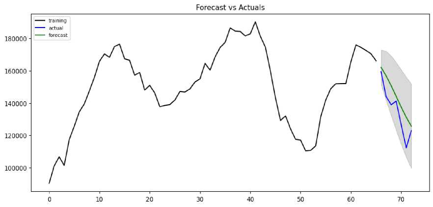
Fig. 4. Actual values and the fitted values of the ARIMA (3, 0, 2) model for births data

As can be seen from Figure 4. that the ARIMA (3,0,2) model analyzed in terms of predicting the uncertainty of future births performs well. Here, there is a high probability that actual birth observations will be within the 95% prediction intervals. In Table 4, the forecasted values of ARIMA (3,0,2) model and the actual values were presented for each year.

Table 4. The predicted values of ARIMA (3, 0, 2) model and the actual values

Year	Actual	Predicted number of births
2016	159464	162100
2017	144041	156772
2018	138982	150576
2019	141179	143917
2020	126571	137226
2021	112284	130935
2022	122846	125449

• So,    ARIMA (3,0,2) model is determined to be the best fit model for the birth data. The prediction of births in Azerbaijan over the next 8 years using the ARIMA (3,0,2) model is calculated, and illustrated in Fig. 5.

• 3.2.    Forecasting the number of deaths data

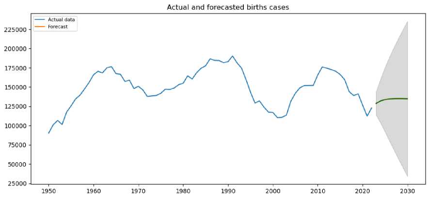
Fig. 5. Prediction the number of births for the next years.

Table 5 shows the forecasting of births for the next years in Azerbaijan (from 2023 to 2030). As can be seen from the Fig.5 and the Table 5, the number of births in the country is expected to increase first and then decrease.

Table 5. Forecasting the number of births for the next eight years in Azerbaijan

Predicted date	Forecated value of births (fc_series)	Minimum prediction (lower_series)	Maximum prediction (upper_series)
2023	128752	113728	143776
2024	132001	103318	160685
2025	133735	91763	175706
2026	134603	79939	189266
2027	134977	68199	201755
2028	135070	56658	213482
2029	135002	45333	224672
2030	134842	34196	235489

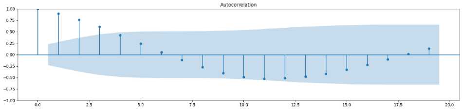
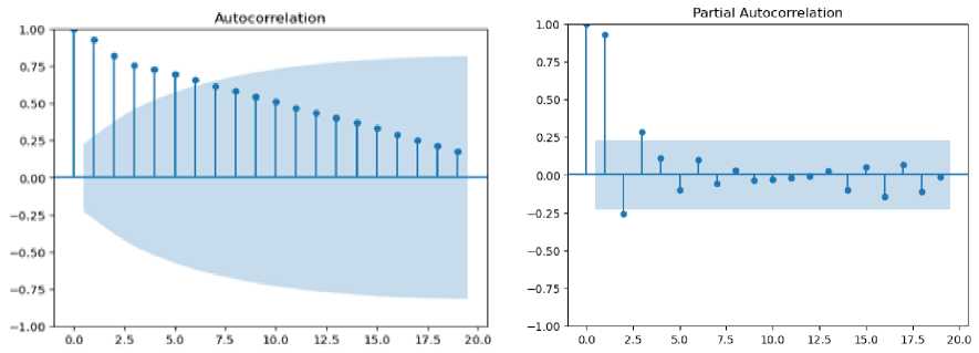
The deaths time series data was plotted on a graph, as shown in Fig.1 (b). As mentioned earlier, ARIMA models usually applied on stationary time series. We first check the stationarity of the time series. Figure 6 indicates that there is a general tendency in the data, so the time series is not a stationary. The time series seems to have an increasing trend for the most part which make it non-stationary. The ACF plot (Fig.6 (a)) is slowly decreasing and has a large number of lags, that is positive, whereas a stationary time series will drop to 0 relatively quick. The PACF plot (Fig.6 (b)) has a first lag of around 2 proving it to be non-stationary.

b)

a)

Fig. 6. The ACF (a) and PACF (b) plots for the death time series.

For further investigation of the stationarity of the time series, ADF and KPSS tests were applied for the training series. The null hypothesis of ADF test is that the data are non-stationary. As mentioned above large p-values indicate the data non-stationarity while small p-values indicate the reverse.

Table 6. p-values of ADF and KPSS for training deaths data series.

Test	ADF Statistic	KPSS Statistic
p-value	0.976	0.01

As shown in Table 6, the p-value of KPSS test is 0.01 (which is less than 0.05), but the p-value of ADF test is 0.976 which is greater than p = 0.05. This indicates that the time series for the deaths is not stationary. The ACF and PACF of the death data decreases slowly which indicates non-stationarity of data. All the above results and plots confirm that the training series are not stationary, and differencing is required for stationarity of data. The autocorrelation functions graphs of the first difference death time series data have been illustrated in Fig. 7.

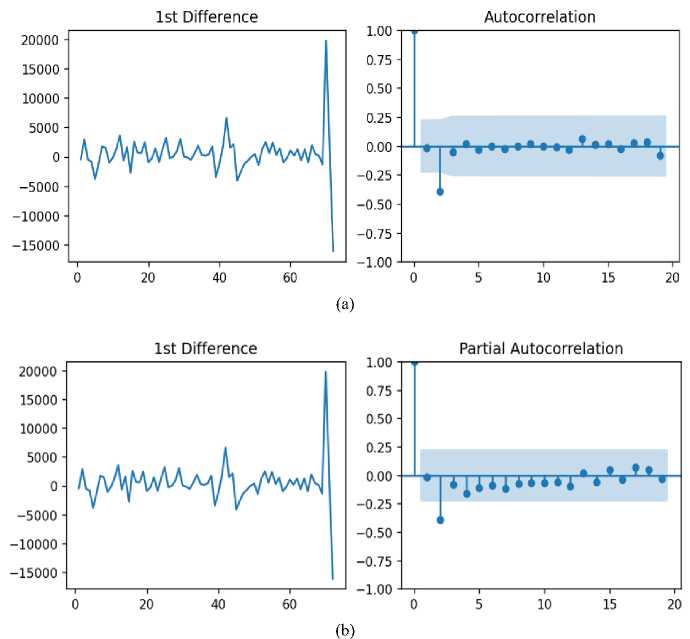
Fig. 7. The ACF (a) and PACF (b) graph of the first order differencing of the death time series

As can be seen from Fig. 7 that the time series is stationary after the first differencing. For further investigation of the stationarity of the time series, ADF and KPSS tests were applied for the training series. The fact that the ADF test result is less than 0.05 also confirms that this series is stationary.

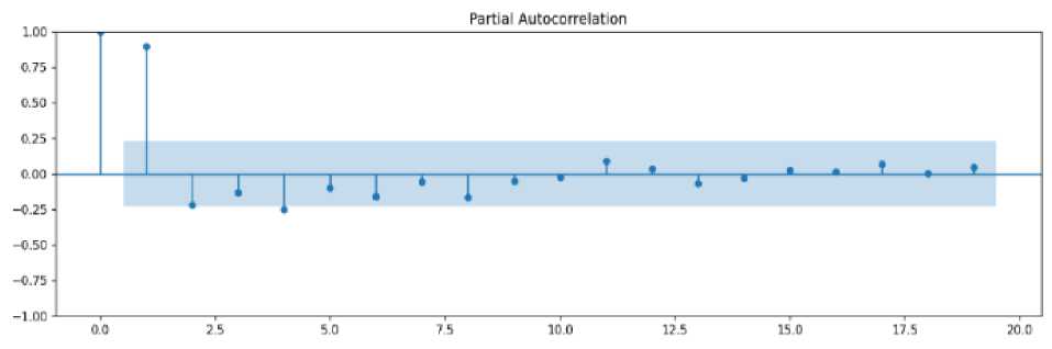
Next step is to find the best-fitted model for first differencing. The p parameter of model is determined by the PACF plot (Fig. 7 (b)), while the q parameter is determined by the ACF plot (Fig. 7 (a)). As can be seen from Fig. 7 (a), only the first lag goes far into the positive zone. For simplicity, we fix the value of q as "0". In the Fig. 7(b), we see two significant lags that the first lag goes far into the positive zone, and another lag goes into the negative zone. Thus, we consider “p” to be 2.

Using the cross-validation method, data 85% were selected as the training set and data 15% were selected as the test set to predict. In this study, the least AIC value is 1381.771, and BIC value is 1387.501 as given in Table 7, and the optimal model is ARIMA (2,1,0) with the lowest MAPE values of 8.89% and RMSE values of 13.9734. The p value (p=0.18) of Ljung–Box test of the ARIMA (2,1,0) model is greater than 0.05. It indicates that the residual of selected model conforms to the characteristics of white noise sequence, and model was suitable for forecasting.

Table 7. Model selection for death data.

Model	AIC	BIC	MAPE	RMSE
ARIMA (1,1,1)	1383.470	1390.300	0.0905	17.2813
ARIMA (0,1,1)	1383.057	1387.611	0.0909	19.5674
ARIMA (1,1,0)	1382.989	1387.543	0.0908	18.8765
ARIMA (2,1,0)	1381.77	1387.501	0.0889	13.9734
ARIMA (2,1,1)	1383.118	1392.224	0 .0906	17.2847

After identification the value of p, d and q, the next step is to estimate the parameters. Accordingly, the parameters of model have been estimated and presented in Table 8.

Table 8. Parameter estimate for the ARIMA (2, 1, 0).

Variable	Coefficient	Standard Error	t-statistic	p-value
AR(2)	-0.1905	0.033	-5.771	0.000

The result of these estimates shows that the AR parameters for ARIMA (2,1,0) of deaths data is statistically significantly different from zero (less than 0.05) and the residuals of selected model conforms to the characteristics of white noise process. Therefore, this model may be used to forecast the deaths. A visual demonstration of the fitted values of the ARIMA (2,1,0) model and actual values for deaths is illustrated in Fig. 8.

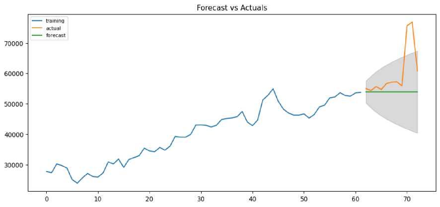
Fig. 8. Actual values and the fitted values of the ARIMA (2,1,0)) model for deaths data

As you can see from Fig. 8, the ARIMA (2,1,0) model predicts a correct forecast. But the model seems to fail in predicting the uncertainty of future deaths. Because there is a high probability that a certain part of the actual mortality observations deviates from the 95% prediction interval.

To improve the prediction accuracy, we find the best model for d=2 (the second differencing) and compare its performance with the previous model. To find the parameters (p and q) of the model, we consider the ACF and PACF for the second differencing (Fig 9). We determine the values of parameters q (q=1) and p (p=2) from the graphs of these functions.

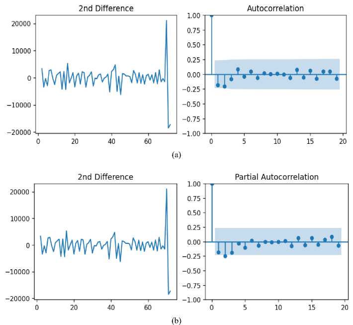
Fig. 9. The ACF (a) and PACF (b) graph of the second order differencing of the death time series

The best suitable ARIMA model for above series was selected based on minimal AIC and BIC values. In this study, the least AIC value is 1373.921, and BIC value is 1382.972 as given in Table 9, and the optimal model is ARIMA (2,2,1) with the lowest MAPE values of 5.51% and RMSE values 8.7316. Using the cross-validation method, data 85% were selected as the training set and data 15% were selected as the test set to predict.

Table 9. Model selection for death data.

Model	AIC	BIC	MAPE	RMSE
ARIMA (0,2,1)	1381.370	1385.895	0.0615	9.8643
ARIMA (1,2,0)	1398.718	1403.243	0.0599	8.8370
ARIMA (1,2,1)	1378.844	1385.632	0.1545	21.1497
ARIMA (2,2,1)	1373.921	1382.972	0.0551	8.7316
ARIMA (2,2,0)	1395.223	1402.011	0.0601	9.4682

After identification the value of p, d and q, the parameters for the ARIMA (2,2,1) of death time series have been estimated and presented in Table 10.

Table 10. Parameter estimate for the ARIMA (2, 2, 1).

Variable	Coefficient	Standard Error	t-statistic	p-value
AR (2)	-0.2894	0.054	-5.404	0.003
MA (1)	-0.9981	0.069	-14.515	0.012

The results of these estimates show that the AR and moving MA for ARIMA (2,1,0) of deaths data is statistically significantly different from zero (less than 0.05), the test statistic is statistically insignificant and the residuals of selected model conforms to the characteristics of white noise process. Therefore, this model may be used to forecast the deaths.

A visual demonstration of the fitted values of the ARIMA (2,2,1) model and actual values for deaths is illustrated in Fig.10.

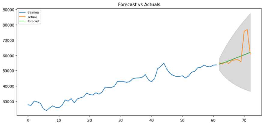
Fig. 10. Actual values and the fitted values of the ARIMA (2, 2, 1) model for deaths data.

As can be seen from Fig 10. that the ARIMA (2,2,1) model analyzed in terms of predicting the uncertainty of future deaths, performs well, unlike the ARIMA (2,1,0) model. Here, there is a high probability that actual death observations will be within the 95% prediction intervals. In Table 11, the forecasted values of ARIMA (2,2,1) model and the actual values were presented for each year.

Table 11. Actual values and the predicted values of ARIMA (2,2,1) model

Year	Actual	Predicted number of deaths
2012	55017	54270
2013	54383	54931
2014	55648	55665

2015	54697	56433
2016	56648	57218
2017	57109	58010
2018	57250	58805
2019	55916	59603
2020	75647	60401
2021	76878	61199
2022	60810	61998

So, ARIMA (2,2,1) can be considered as the best fit model and can be further used to generate the forecasts. In Table 12, are presented the forecasts for death of the next eight years estimated with the ARIMA (2,2,1). Also, a visual demonstration of the forecasts of the ARIMA (2,2,1) is illustrated in Fig. 11.

Table 12. Forecasting the number of deaths for the next eight years (2022-2030) using ARIMA (2,2,1)

Predicted date	Forecated value of deaths (fc_series)	Minimum prediction (lower_series)	Maximum prediction (upper_series)
2023	62083	55277	68890
2024	63126	54867	71385
2025	64014	55139	72889
2026	64799	55633	73964
2027	65514	56202	74826
2028	66182	56792	75573
2029	66820	57385	76254
2030	67436	57975	76898

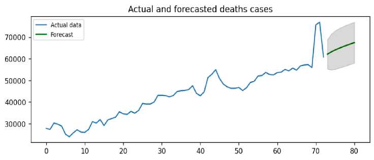
Fig. 11. Forecasting the number of deaths for the next eight years (2022-2030)

So, ARIMA (2,2,1) model on death shown that number of deaths will continue to increase by next eight years in country.

The decline in birth rates and increases in mortality rates may lead to a future population decline, which could negatively affect the country's demographic and economic development. With population decline, the number of older people increases, while the number of young people of working age decreases. This leads to labor shortages, the collapse of the pension system, and an economic slowdown. The decline in the working age population reduces economic production and tax revenues. This makes it difficult to sustain social security systems. The proposed models fit properly with the data used in this research, and show a valid prediction that present a low percentage error. Therefore, it can be considered reliable for decision making aimed at timely prevention of the demographic challenges that the country may face.

4.    Conclusion

In the study, the best-fitted ARIMA models for birth and death were estimated and the models were used to forecast of number of births and deaths the next eight years, respectively. Since the original birth data used in the study were stationary, differencing was not required. However, since the death data were non-stationary, we used (first-order and second-order) differencing to bring it into stationarity. It was found that the best model selected in the first differencing (d=1) was unsuccessful in predicting uncertainties. To improve the prediction accuracy, we found the best model for d=2 and found that its performance was superior to the previous model. This shows that the performance of the ARIMA model depends on the parameters p, d and q. The prediction results of the models are evaluated MAPE and RMSE, the prediction capabilities of the models are compared. These models fit properly with the data used in this research, and show a valid prediction that present a low percentage error. According to the values predicted by the ARIMA (3,0,2) model, the number of births in the country is expected to increase first and then decrease. There is expected to increase in the number of deaths in the country over the next eight years according to the ARIMA (2,2,1) model on death.

Thus, by effectively using the ARIMA model, reliable predictions of birth and death rates for the near future can be obtained, which can be useful for demographers and government officials, especially health and social sector officials, in timely and systematic management of child health indicators, providing financial support to families, determining the sustainability of pension and social security systems, and strategic planning. ARIMA models are not explicitly designed to capture seasonal patterns in the data, which can lead to inaccuracies in forecasting for datasets with significant seasonal variations. For this purpose, it is planned to use the SARIMA model and machine learning methods in future research.