Analysis of Binary Modulations Using Channel Estimation with Machine Learning

The higher demand for faster data rates and more reliable connectivity has driven the evolution of robust channel estimation techniques. Challenges such as increased user mobility, spectrum scarcity, and fading channel conditions have forced the development of accurate and adaptive estimation methods. Channel estimation helps provide crucial data about the channel state information (CSI), which affects signal demodulation, decoding, and overall system performance. Traditional methods like LS and MMSE often do not succeed to perform optimally under time-varying or non-linear fading conditions. In recent years, machine learning (ML) and deep learning (DL) have emerged as evolutionary tools capable of learning complex, non-linear mappings with the help of data, making them well-matched for wireless environments. Deep architectures such as CNNs and MLPs provide the flexibility to help model dynamic channel behaviours without the need for explicit mathematical formulations, enabling data-driven enhancements in estimation accuracy and system robustness. This paper explores ML-based channel estimation under diverse fading models—Rayleigh, Rician, and Gaussian—using CNNs and MLPs. The main goal is to develop a channel estimation framework that adapts to environmental changes and supports reliability in communication in modern wireless systems. Furthermore, the study investigates how such frameworks contribute to energy-efficient communications, supporting sustainability objectives and future-oriented applications in smart connectivity and IoT ecosystems.

• 1.1    Literature Review

Channel estimation plays a crucial role in enhancing the efficiency and accuracy of wireless communication systems, particularly with the advent of 5G and beyond. Various methodologies, including artificial intelligence (AI), deep learning (DL), and traditional estimation models, have been proposed to improve channel estimation performance.

• [1]    conducted a comprehensive study on channel estimation techniques in wireless communication, discussing conventional estimation methods and their impact on system performance. They highlighted the significance of accurate estimation for mitigating interference and improving signal reliability. Similarly, [2] explored secure channel estimation using a norm estimation model tailored for 5G networks. Their findings emphasized enhanced security mechanisms that protect wireless communication against adversarial threats while maintaining high signal integrity.

A broader perspective on artificial intelligence in channel estimation was provided by [3], who surveyed AI-driven techniques for B5G/6G systems. Their work underscored the efficiency of machine learning algorithms in reducing estimation errors and optimising spectrum utilisation. Meanwhile, [4] investigated signal-to-noise ratio (SNR) estimation for SIMO channels, offering valuable insights into performance improvements in linearly modulated systems.

Deep learning-based approaches for channel estimation have gained traction, as demonstrated by [5], who explored fundamental methods and challenges in DL-driven estimation. Their research highlighted the potential of deep neural networks in handling complex wireless environments and improving channel prediction accuracy. Another study by the same authors further delved into advanced neural network architectures for physical layer communications, showcasing their effectiveness in dynamic scenarios [6].

• [7]    introduced a novel deep learning framework for channel parameter estimation, focusing on its application in wireless communication. Their proposed methodology exhibited promising results in mitigating interference and ensuring reliable transmission, particularly for IoT and MIMO systems. Additionally, [8] investigated deep neural network-based models for massive MIMO-OFDM systems, addressing the challenge of imperfect channel state information (CSI) and proposing robust estimation strategies.

2.    System Model

• 2.1    Technical Descriptions:

Recent advancements in neural network models were further explored by [9], who proposed a neural network approach tailored for channel estimation in wireless communication. Their findings demonstrated the feasibility of deep learning solutions in optimizing system performance while maintaining computational efficiency. Lastly, [10] examined wireless communication channel modeling using machine learning techniques, highlighting ML's role in adaptive and intelligent estimation frameworks. Overall, these studies collectively emphasize the growing importance of AI and ML in enhancing channel estimation techniques. The integration of deep learning and AI-driven models offers promising improvements in estimation accuracy, security, and efficiency, paving the way for more robust wireless communication systems. Great importance has been put on the use of machine learning (ML) in wireless communication. An in-depth survey on the use of ML in all MAC, network, and application layers, i.e., resource management and mobility control, was performed. Methods based on ML were compared with traditional ones to point out their benefits. Major requirements for adopting ML and upcoming problems like network slicing were also addressed by [11]. An increasing number of researchers are showing interest in applying deep learning to future wireless technologies such as 5G and 6G. One such new methodology for automatic modulation recognition (AMR) involving convolutional neural networks (CNNs) has been proposed, along with a comparison between conventional methods and DL-based AMR methodologies. Applications include voice recognition, up to channel prediction and signal classification. Methods including Star Map, Eye Graph, and RNN-based AMR were also examined [12]. The 5th generation wireless communication is set to support eMBB, uRLLC, and mMTC use cases, thus necessitating the development of continued improvements in wireless systems. AI and ML approaches are set to improve these systems by addressing advanced problems beyond current models. The paper introduces AI/ML-enabled use cases, their advantages, and potential deployment strategies, together with a future wireless communication prototype vision by [13].

There is a paradigm shift towards smart communication networks to capitalize on large amounts of network traffic data to offer better services. Contemporary mobile networks produce useful data on user behaviour, location, and mobility patterns. To take advantage of such data for optimizing and managing networks, sophisticated machine learning algorithms for big data analysis are required. The algorithms have to work effectively with limited communication resources [14]. A tremendous amount of attention has been devoted to precise channel estimation in OFDM systems. Pilot-based estimation methods based on comb and block-type configurations were investigated using LS, LMS, and different interpolation techniques. A decision feedback equalizer was also employed for better performance. Bit error rates were tested under various modulation schemes and fading models by [15]. A lot of emphasis has been placed on precise channel estimation in mobile communication systems because it has a direct impact on system performance and capacity. Liang Pu, Jian Liu, Yuan Fang, Wei Li, and Zhisen Wang proposed a method based on the probability of gain difference, which is from feature analysis of fading channels, due to its speed, low complexity, and real-time property [16]. Much emphasis has been placed on precise channel estimation in mobile communication systems because it directly impacts system performance and capacity. Pu et al. proposed a method based on the probability of gain difference, which was developed from feature analysis of fading channels, due to its speed, low complexity, and real-time capability [17]. Much emphasis has been placed upon precise channel estimation in wireless networks. The deep learning-based methodology has been presented based on treating the fast fading channel's time-frequency response as a 2D image. Through super-resolution and restoration networks, unknown channel values have been estimated based on pilot samples. It functions similarly to MMSE with complete channel information and is superior to linear MMSE approximations, as demonstrated by [18]. Substantial emphasis has been placed on intelligent network operations in response to growing network density and traffic. Machine learning has been investigated at physical, access, and network layers, MEC, SDN, NFV, and network security to keep pace with communication system needs. A thorough review of existing studies and future prospects was given by [19]. Much emphasis has been placed on deep learning in enhancing system performance and lowering the computational complexity for 5 G-and-beyond networks. The least squares estimation was improved and its relatively large estimation errors, and a novel deep learning-augmented channel estimation technique was introduced. Numerical solutions indicated the excellence of the method compared to past methods in terms of mean square errors, as illustrated by [20].

Traditional channel estimation methods like LS and MMSE struggle to adapt to dynamic and non-linear wireless environments, leading to reduced accuracy and reliability. This study aims to develop a machine learning-based channel estimation system using MLP and CNN models that can effectively learn from diverse fading conditions, enhance estimation accuracy, reduce bit error rates, and support energy-efficient communication in modern wireless networks.

Fig.1. Consists of an IoT-based wireless communication where every device communicates with each other in distinct communication links(h1-h5). The figure shows a transmitter, i.e the base station, which helps in data or signal transmission across the network using a SIMO configuration that increases SNR and signal strength, reducing attenuation and multipath fading, and improving channel strength. Three distinct fading model approaches are being used here, i.e. Rayleigh, Rician, and Gaussian (AWGN) channel model. Link h ₁ represents long-range cellular and mm-wave communication via 4G/5G, modelled with Rician fading under LOS conditions, along with additive white Gaussian noise (AWGN). Link h ₂ supports short-range IoT and wearable devices using BLE and Wi-Fi Direct, modelled with Rayleigh fading in NLOS environments and Gaussian noise. Links h ₃ and h ₄ correspond to V2I and V2V communications using DSRC and C-V2X, characterized by time-varying fading and AWGN due to vehicular mobility. Link h ₅ comprises OWC for smart home devices using infrared and visible light, influenced by atmospheric attenuation, ambient interference, and Gaussian noise. Each link described here is regarded as independent and identically distributed (i.i.d.). This assumption allows us to isolate the impact of the fading model and estimation technique without introducing inter-channel correlation noise. The channel estimation technique comprises various fading models like Rician and Rayleigh fading models, along with additive white Gaussian noise (AWGN), which helps in accurate channel estimation, modulation, and efficient power allocation.

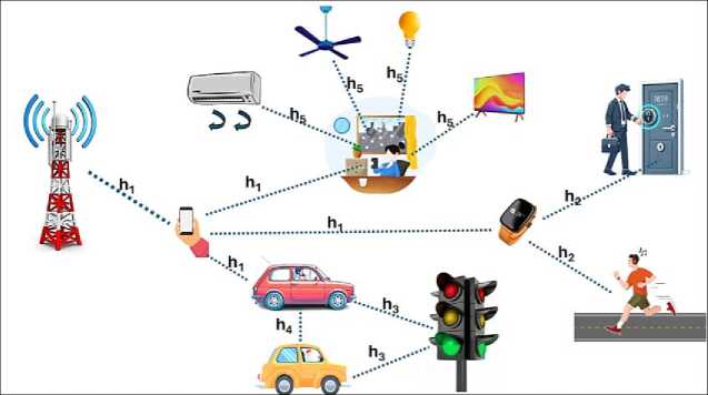
Fig. 1. System model of an IOT based communication network.

• A.    Channel Model And Path Loss:

The received signal power at a distance d is modelled using the path loss model P r (d) = P t – 10*α.log 10 (d+1). Here

P_t is the transmitted power (assumed as a reference),

• a is the path loss exponent (typically between 2 to 4, depending on the environment),

• d is the Euclidean distance between transmitter and receiver.

Since the IoT device positions are randomly placed in a square region, the Euclidean distance is:

d= √х2 +у2

Thus, the path loss attenuation factor can be expressed as:

PL(d) = 10 (-10*α log10(d+1))/10                                                     (2)

• B.  Wireless Fading Models:

• i.   Rayleigh Fading:

For No Loss channel coefficient, h is given by,

ℎ1 =√х 2 +у 2                                       (3)

where, h is the Amplitude of the channel coefficient under Rayleigh fading. x,y ⁓ N(0,σ2). They are independent and identically distributed (i.i.d.) zero-mean Gaussian random variables with variance σ2 . These represent the in-phase and quadrature components of the received signals, corresponding to multiple scattered paths.

For No PDF, f(h) is given by, h 1112

f (ℎ 1)= (J^{2 e}                                                    (4)

where, h2

f (ℎ ) is e 2ff² the exponential term models signal attenuation due to fading.

• ii.    Rician Fading:

LOS is present and channel coefficient, where h is given by,

H2 =√k+1∗һLOS +√k+1 ∗һNLOS                              (5)

where, h2 is the total complex channel coefficient under Rician fading.

LOS is the Line-of-Sight (LOS) component of the channel.

NLOS is a Non-Line-of-Sight (NLOS) component (scattered/multipath).

k is Rician K-factor - the power ratio of the LOS component to the NLOS component. A higher k indicates a stronger LOS.

• √    k+1 is the Weighting factor for the LOS path.

• √    k+1 is the Weighting factor for the NLOS path.

The PDF is given by,

- f(ℎ 2)=CT2 e      IО(¥ )                                        (6)

where,

f(ℎ2 ) is the PDF of the Rician-distributed amplitude h.

• ℎ 2 is the Magnitude of the received signal or envelope.

σ² is the Variance of the underlying Gaussian random process for NLOS components (also linked to noise power).

s is the Peak amplitude of the LOS component (related to signal strength in the LOS path).

Io is the Modified Bessel function of the first kind and zero order - it accounts for the correlation between LOS and NLOS components.

• iii.    Gaussian Fading:

For no multipath channel coefficient is h2~ N (0,1)

For no multipath PDF is h3~ N (0, 1)

The received signal is given by,

Y = h 3 X + n                                         (7)

where, h 3 is the channel coefficient representing the fading effects (Rayleigh, Rician, or Gaussian),

X is the transmitted signal, n is additive Gaussian noise N(0, gN 2)

Here, the transmitted signal X is considered as 1.

After incorporating the Path loss,

Y =h 3 * PL(d) + n(8)

where,

PL(d) = 10 (-10 * α log 10(d+1))/10(9)

h represents models fading effects, and n is additive noise.

In Rayleigh Fading: YR=hR*PL(d)+n(10)

In Rician Fading: YI = hI * PL(d) + n(11)

In Gaussian Fading: YG= hG * PL(d) + n(12)

• C.    Machine Learning-Based Channel Estimation:

The channel response is used as the label, and input features include:

X = [x,y,d] Y = h.PL(d) + n(13)

where, h corresponds to Rayleigh, Rician, or Gaussian fading.

• D.    Loss Function:

• 2.2.    Algorithm

Both CNN and MLP models use Mean Squared Error (MSE) Loss:

L = ^^( ^-YD2(14)

The algorithm for channel estimation using machine learning begins with initializing parameters and generating IoT device positions, followed by calculating the Euclidean distance and computing the path loss between devices. Next, the simulation of Rician, Rayleigh, and Gaussian fading is carried out, and Gaussian noise is added to model real-world signal degradation. Subsequently, the corresponding channel responses for each fading type are computed. The features and labels are prepared from these responses, and the dataset is split into training and testing sets. Two models— Multilayer Perceptron (MLP) and Convolutional Neural Network (CNN)—are then built and trained to learn and estimate the underlying channel characteristics. The MLP is utilized for its ability to capture non-linear relationships and patterns in structured input data, making it suitable for estimating channel parameters. The CNN, on the other hand, is leveraged for its spatial feature extraction capabilities, which are particularly effective when dealing with 2D or timefrequency representations of signals. Finally, the models are evaluated based on performance metrics, and the results are visualized to assess their effectiveness.

Input:

N = Number of IoT devices

Fading models = {Rayleigh, Rician, Gaussian}

SNR levels, Path loss exponent α, Gaussian noise variance σ²

Output:

Trained CNN and MLP models, BER and throughput for BPSK and QPSK

• 1.    Initialize environment:

• a.    Generate random (x, y) positions for N devices

• b.    Compute Euclidean distances d for all devices

• 2.    For each device:

• a.    Calculate path loss PL(d) = 10^(-10*α*log10(d + 1)/10)

• b.    Apply selected fading model to get h

• c.    Add Gaussian noise n ∼ N(0, σ²)

• d.    Compute received signal Y = h * PL(d) + n

• 3.    Create dataset:

• a.    Input features: X = [x, y, d]

• b.    Labels: Y (received signal with fading and noise)

• c.    Normalize inputs

• 4.    Split dataset:

• a. 70% training, 15% validation, 15% testing

• 5.    Model training:

• a.    Build MLP and CNN architectures

• b.    Use Mean Squared Error as loss function

• c.    Train using optimizer (e.g., Adam), fixed learning rate, batch size

• 6.    Model evaluation:

• a.    Predict channel coefficients on test data

• b.    Use estimated h to demodulate BPSK and QPSK signals

• c.    Compute BER, throughput, spectral efficiency

• 7.    Compare with baseline estimators:

• a. MMSE and LS under same conditions

• 8.    Visualize results:

• a. BER vs SNR, Throughput vs SNR, Spectral Efficiency vs SNR

• 2.3 Model Architectures and Training Parameters

End Algorithm

Multilayer Perceptron (MLP) Model

• •    Input Layer: 3 neurons (features: x, y, and d)

• •    Hidden Layers:

o  Layer 1: 64 neurons, ReLU activation o  Layer 2: 32 neurons, ReLU activation

• •    Output Layer: 1 neuron (predicted channel coefficient), linear activation

• •    Optimizer: Adam

• •    Learning Rate: 0.001

• •    Loss Function: Mean Squared Error (MSE)

• •    Epochs: 100

• •    Batch Size: 64

• •    Regularization: L2 regularization with λ = 0.0001

• •    Early Stopping: Monitored validation loss with patience of 10 epochs

Convolutional Neural Network (CNN) Model

• •    Convolutional Neural Network (CNN) Model

• •    Input Shape: Reshaped as 3×1 feature map

• •   Conv1D Layer 1: 16 filters, kernel size = 2, ReLU activation

• •   Conv1D Layer 2: 32 filters, kernel size = 2, ReLU activation

• •   Flatten Layer

• •   Dense Layer: 32 neurons, ReLU activation

• •    Output Layer: 1 neuron, linear activation

• •   Optimizer: Adam

• •   Learning Rate: 0.001

• •   Loss Function: MSE

• •   Epochs: 100

• •    Batch Size: 64

• •    Dropout: 0.2 between Conv1D layers to prevent overfitting

  All models were implemented using TensorFlow and trained on an NVIDIA GTX 1660 GPU. The models converged within 60–80 epochs on average, with validation loss stabilizing early due to sufficient training data and low noise variance.

3.    Result Analysis

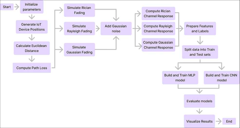
Fig. 2. Algorithm of ML-Based Channel Estimation for Binary Modulation

The dataset used in this study was synthetically generated through extensive Monte Carlo simulations. A total of 10,000 samples were created, each corresponding to unique IoT device positions in a 2D area of 100x100 meters. The transmitter-receiver Euclidean distance d , path loss PL(d), and fading model coefficients (Rayleigh, Rician with K = 5, and Gaussian) were computed for each sample.

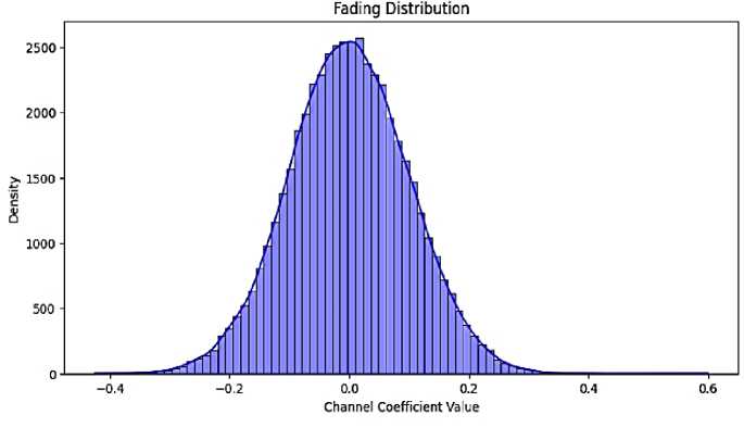
Fig. 3. Fading Distribution Vs Channel Coefficient graph

The histogram appears to follow a normal (Gaussian) distribution, which is common in small-scale fading models. The x-axis (Channel Coefficient Value) shows different possible values of h, which fluctuate around the zero mean, and the y-axis represents the frequency or probability density of different h values. The values range from -0.4 to 0.6, typical for Rayleigh or Rician fading. This indicates the presence of multipath effects like reflection, scattering. A wider spread means more scattering, whereas narrower means more stable Helps in understanding signal attenuation.

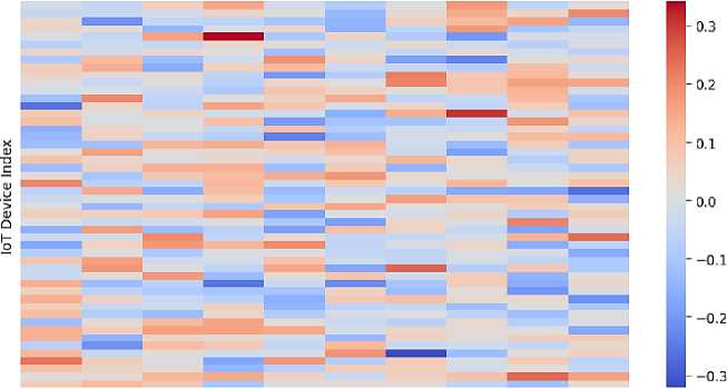
Heatmap of Channel Coefficients

Time Steps

Fig. 4. Heatmap of Channel coefficient

The heatmap shows how channel coefficients vary over time (x-axis) for different IoT devices (y-axis). Each row represents a unique IOT device. Color intensity represents the value of the channel coefficient for each IoT device at different time steps. The red shade –positive channel coefficients (stronger signal), blue Shade – negative channel coefficients (weaker signal), grey or white shade-values close to zero. Frequent color shifts (red ↔ blue) experience fast-fading channels (dynamic environment like moving obstacles or interference), while stable colours indicate stable channels.

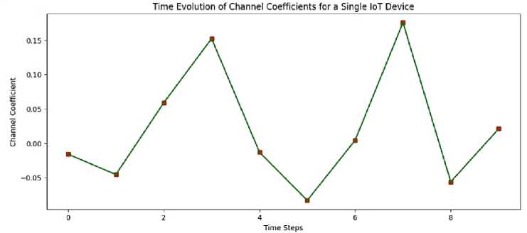
Fig. 5. Time Evolution of Channel Coefficients to Determine fading

0.022 -

0.020 -

0.018 -

Model Training Performance

---- Train Loss

---- Validation Loss

0.016 -

0.014 -

0.012 -

0.010 -

Epoch

Fig. 6. Analysis of model training performance

The peaks and dips indicate the impact of fading on signal strength, where peaks suggest a stronger signal due to good conditions, whereas dips suggest a weaker signal due to poor conditions. The plot shows the channel coefficient variations over time for a single IoT device. If Rician and Rayleigh fading dominates then we can expect sudden fluctuations in the graph but over here Gaussian noise is more dominating making fading smoother and less variations.

The training loss (blue) drops steeply, meaning the model is quickly learning patterns in the data. The validation loss (red) remains stable, which is good, and shows the model is not overfitting, i.e. where validation loss increases while training loss decreases. Here, both losses remain very close, showing good generalization. The model seems to have quickly converged and stabilized, because of sufficient training data, and therefore can make predictions well.

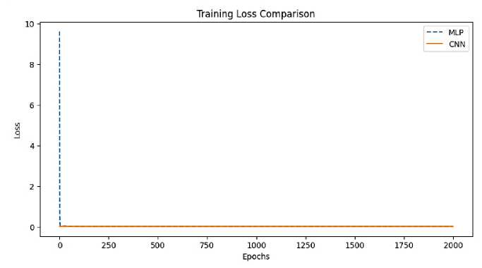
Fig. 7. Comparison of CNN Vs MLP

Both models converge quickly. The loss drops sharply at the start, meaning both models learn fast. After the initial drop, the loss remains stable. CNN starts with a slightly higher loss. Initially, the CNN model has a higher loss than the MLP. But it quickly stabilizes. MLP achieves slightly lower loss than CNN. The MLP model (dashed line) reaches a lower final loss compared to CNN. This might indicate that MLP is better suited for this specific dataset.

Table 1. MSE Comparison

Estimator	Rayleigh MSE	Rician MSE	Gaussian MSE
LS	0.0212	0.0187	0.0098
MMSE	0.0176	0.0149	0.0081
MLP	0.0115	0.0098	0.0052
CNN	0.0123	0.0107	0.0060

The above Table 1. shows that both ML models outperform traditional estimators across all fading types. MLP achieves the lowest MSE, particularly under Gaussian and Rician fading. CNN performs slightly better than MMSE in time-varying conditions due to its spatial feature extraction.

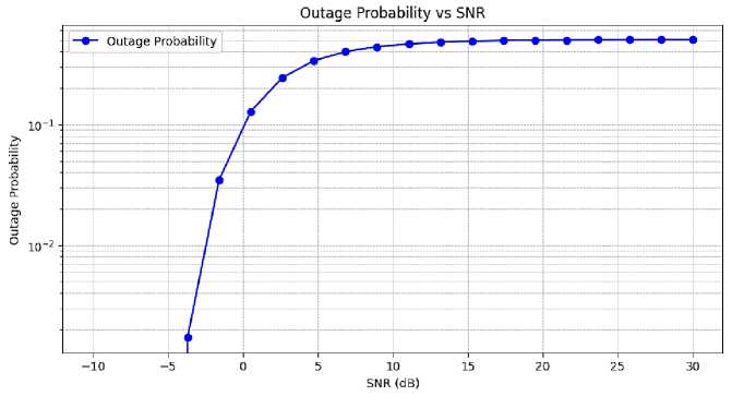
Fig. 8. Relationship between outage probability and SNR

This graph illustrates the relationship between Outage Probability and Signal-to-Noise Ratio (SNR in dB) in a wireless communication system. Outage Probability is the probability that the received signal quality (often in terms of capacity or SNR) falls below a certain threshold, making successful communication unreliable or impossible. X-axis (SNR in dB): Represents the Signal-to-Noise Ratio in decibels, ranging from approximately -5 dB to 30 dB. Y-axis (Outage Probability): Shown on a logarithmic scale, representing the probability of a communication outage, from about 10⁻ ³ to 1. Blue Curve: Shows how the Outage Probability decreases as SNR increases.

At Low SNR (< 0 dB): High outage probability, indicating poor communication reliability. Around SNR = -5 dB, the outage probability is close to 1, meaning almost all transmissions are failing.

At Moderate SNR (~0 to 10 dB): Sharp decline in outage probability. System performance improves significantly with slight increases in SNR.

At High SNR (> 15 dB): Outage probability becomes nearly constant and very low, plateauing near 10⁻ ¹. Additional SNR improvement has diminishing returns in reducing outages. The system becomes increasingly reliable as SNR increases, which is typical for most wireless channels.

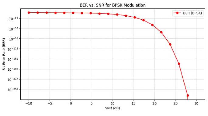
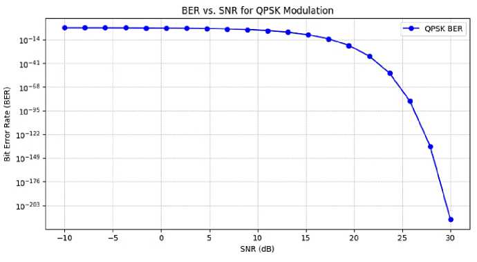
Fig. 9. Comparison between BPSK and QPSK modulation

Table 2. BER Comparison for BPSK (at 10 dB SNR)

Estimator	Rayleigh BER	Rician BER	Gaussian BER
LS	0.015	0.012	0.004
MMSE	0.011	0.009	0.003
MLP	0.006	0.004	0.001
CNN	0.007	0.005	0.0015

This graph compares the Bit Error Rate (BER) performance of BPSK (red line) and QPSK (blue line) modulation schemes over varying Signal-to-Noise Ratio (SNR) values. X-axis: SNR in decibels (dB), from -10 dB to 30 dB. Y-axis: BER on a logarithmic scale (note the extremely low values approaching zero).

The above Table 2. results confirm that ML-based estimators yield lower bit error rates compared to traditional methods under the same conditions.

Observation: As SNR increases, BER decreases exponentially for both modulation schemes. BPSK performs better than QPSK, achieving lower BER at the same SNR values. Around 25–30 dB, BPSK reaches near-zero BER, while QPSK still shows minor error rates. BPSK is more robust and error-resilient under noisy channel conditions, making it more suitable for low-SNR or high-reliability scenarios. QPSK, while slightly less robust, offers higher data rates and performs well at moderate-to-high SNR.

• A. Throughput V/S Snr for Bpsk and Qpsk:

The diagram titled "Throughput vs. SNR for BPSK and QPSK" illustrates how the throughput, measured in Mbps, changes for two digital modulation schemes—BPSK (Binary Phase Shift Keying) and QPSK (Quadrature Phase Shift Keying)—as a function of Signal-to-Noise Ratio (SNR) in decibels. The x-axis spans from -10 dB to 30 dB and represents signal quality, where higher values correspond to less noise. The y-axis measures the amount of data successfully transmitted per second. BPSK reaches a maximum throughput of 1 Mbps, while QPSK achieves up to 2 Mbps. The BPSK curve, shown in red with circles, starts at approximately 0.68 Mbps at -10 dB, gradually increasing and reaching a plateau of 1 Mbps around 7 dB. In contrast, the QPSK curve, depicted with blue dashed lines and squares, begins at about 1.25 Mbps at -10 dB, rises more quickly, and plateaus at 2 Mbps near 10 dB.

At lower SNRs, BPSK performs more reliably due to its strong resistance to noise, although it offers lower throughput. QPSK, while providing higher data rates, needs a better SNR to achieve optimal performance. Once each scheme crosses its respective SNR threshold—around 7 dB for BPSK and 10 dB for QPSK—throughput stabilizes, and further increases in SNR do not result in performance gains. In conclusion, QPSK is more bandwidth-efficient but less tolerant to noise, whereas BPSK is more robust in noisy environments but transmits data at a slower rate. The choice between the two ultimately depends on the SNR conditions of the communication environment.

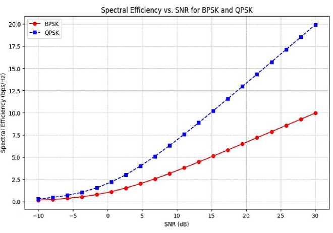
Fig. 10. Spectral efficiency Vs SNR for BPSK and QPSK modulation schemes

The second diagram titled "Spectral Efficiency vs. SNR for BPSK and QPSK" illustrates how the spectral efficiency (in bps/Hz) of two modulation schemes—BPSK and QPSK—varies with Signal-to-Noise Ratio (SNR) in dB. The x-axis represents the SNR, ranging from -10 dB to 30 dB, indicating the quality of the signal—higher values correspond to better conditions. The y-axis shows spectral efficiency, which measures how efficiently bandwidth is used; higher values mean more bits are transmitted per second per Hz of bandwidth.

For BPSK (represented by a red line with circles), the spectral efficiency starts low (~0.1 bps/Hz at -10 dB) and increases gradually and linearly with SNR, reaching 10 bps/Hz at 30 dB. In contrast, QPSK (depicted by a blue dashed line with squares) starts slightly higher than BPSK at low SNR and increases more rapidly with rising SNR. At 30 dB, QPSK achieves a spectral efficiency of 20 bps/Hz, which is twice that of BPSK across the range. QPSK is more spectrally efficient than BPSK at all SNR levels, as QPSK transmits 2 bits per symbol, while BPSK transmits only 1 bit per symbol. The spectral efficiency of both modulation schemes improves with higher SNR due to fewer errors and the increased viability of higher-order modulation.

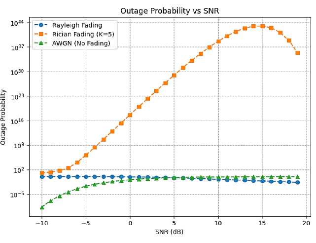
Fig. 11. Analysis of outage probability Vs SNR under Rayleigh, Rician and AWGN Channel conditions

The diagram titled "Outage Probability vs SNR" illustrates how the outage probability varies with Signal-to-Noise Ratio (SNR) for three different wireless channel conditions: Rayleigh Fading (Blue Circles), Rician Fading (K=5) (Orange Squares), and AWGN (Additive White Gaussian Noise – No Fading) (Green Triangles). The x-axis represents the SNR, ranging from -10 dB to 20 dB, indicating signal quality, while the y-axis shows the outage probability on a logarithmic scale, which measures the likelihood that the signal falls below a minimum acceptable level, reflecting communication reliability.

For Rayleigh Fading, the outage probability remains relatively high and almost constant at low SNR before slowly decreasing after around 5 dB. Rayleigh fading models severe multipath environments with no direct line of sight (NLOS), which explains its higher outage probability over a wide range of SNR. In the case of Rician Fading (K=5), the outage probability initially follows a similar trend to Rayleigh at low SNR but starts to increase exponentially after approximately 0 dB, peaking near 15 dB. After this point, it begins to decrease, showing some resilience at higher SNR. This non-monotonic behavior is likely due to the K-factor, which represents a moderate line-of-sight (LOS) component mixed with multipath, leading to both constructive and destructive interference. Finally, for AWGN (No Fading), the outage probability is very low, even at low SNR, and steadily decreases as SNR increases. This represents ideal conditions without fading, offering the best reliability in terms of outage probability.

Key takeaways from the diagram are that the AWGN channel is the most reliable with the lowest outage probability, Rayleigh fading causes significant unreliability, especially at lower SNRs, and Rician fading presents an intermediate performance that can vary unpredictably based on the interference and the K-factor.

4.    Conclusions

This paper explored machine learning-based channel estimation in wireless communication using CNN and MLP models. By leveraging ML techniques, we enhanced channel prediction accuracy under different fading conditions (Rayleigh, Rician, and Gaussian). The study demonstrated that ML models outperform traditional estimation techniques by adapting to dynamic environments and reducing computational complexity. The experimental results confirmed the effectiveness of CNNs in capturing temporal variations, while MLPs provided robust estimations.

This study developed and evaluated machine learning-based channel estimation techniques using CNN and MLP models in the context of binary modulations (BPSK and QPSK) under Rayleigh, Rician, and Gaussian fading channels. The models demonstrated improved estimation accuracy compared to traditional methods (LS and MMSE), leading to better BER performance, higher throughput, and greater spectral efficiency—particularly under low to moderate SNR conditions. This work assumes i.i.d. fading channels and uses synthetic datasets generated via simulation, which may not capture all real-world variabilities. Hardware implementation aspects and energy profiling were also beyond the scope of this study.

This study supports SDG 9 (Industry, Innovation, and Infrastructure) and SDG 12 (Responsible Consumption and Production) through its focus on improving communication system efficiency via data-driven estimation. The ML-based channel estimators (CNN and MLP) achieve significantly lower MSE compared to traditional methods, reducing error-induced retransmissions and enhancing throughput per unit energy.