Analysis on Image Enhancement Techniques

Feature Extraction is the crucial module with respect to particular application. These applications are classified into different categories and these are Face Recognition (FR) [1-8], Texture Investigation (TI) [9] and Object Analysis (OA) [10]. If the extracted features are not effective than classified results are not up to the mark. Feature extraction step is categorized in global and local sections. In global, the algorithm [11, 12] works on full image and then extracted features are fed into the classifier to judge the performance of global feature. In local, the algorithms [13, 14] operate on crucial image parts (such as nose, eyes, mouth, forehead, lips) which are joined entirely to make the full feature size. These local methods are much efficient in various image transformations as literature suggests. The image transformations include the interpersonal and intrapersonal variations. As intrapersonal is the major problem in achieving the discriminativity therefore it should be deal with great care prior to developing the algorithm. Some intrapersonal variation includes light, noise, blur, emotion, pose, corruption and occlusions. In contrast to global, the local ones generally build’s large feature size. Therefore some global method should be utilized for reducing the feature size of local method. The compact method produces far better accuracy as compared to the original large feature size. Therefore the integration of global and local methods proves out much impressive than either of them. As this paper is all about image pre-processing therefore the feature extraction is not discussed in detail. It is noticed from literature that utilization of pre-processing algorithms [15, 16] improves the recognition rates. By taking motivation from their various pre-processing techniques are studied and tested.

Image Enhancement is the crucial segment of image pre-processing. Numerous IET persists in literature to improve the image quality. The image enhancement concept is to improve the image intensity and eliminate noise as much as possible. Several image enhancement techniques and noise removal filters are existing to accomplish this task. After image enhancement is accomplished then various image quality measures are deployed for evaluation. The image quality measures perform image compression, feature extraction, image restoration and image display. Image Quality Measures are classified into three distinct categories and these are FRBIQM, No RBIQM (NRBIQM) and Reduced RBIQM (RRBIQM). In FRBIQM, full reference image is used for image processing. In NRBIQM, no reference image is utilized for image processing. In RRBIQM, a portion of the reference image is utilized for image processing. This paper discusses about IET and the FRBIQM [17-19]. Some introduction regarding IET is discussed earlier. The detailed elaboration is discussed latter on. The short introduction with regard to FRBIQM is illustrated from the next paragraph. The complete details are given latter.

FRBIQM are further classified into Pixel DBIQM (PDBIQM), Edge BIQM (EBIQM) and Corner BIQM (CBIQM). PDBIQM include Mean Square Error (MSE), Peak Signal to Noise Ratio (PSNR), Signal to Noise Ratio (SNR), Normalized Absolute Error (NAE), Structural Content (SC), Maximum Difference (MD), Average Difference (AD), Laplacian Mean Square Error (LMSE), Normalized Cross Correlation (NCC) and Image Fidelity (IF). All these quality measures are illustrated, and then by using sample image and distorted image these measures are computed. These measures evaluate the performance between the original and the distorted image. Edge Based Image Quality Measures (EBIQM) are very crucial for extracting the features. If the sample images are deteriorated from various unwanted details (noise). Then it becomes essential to deploy one or two edge quality measures (best among all) so that edge features are extracted effectively. With the deployment of these edge based quality measures the noise is suppressed and crucial elements are evolved. The edge is the crucial element pertaining to the feature extraction. The numerous edge based operators persist in literature are Robert, Prewitt, Sobel, Canny and Laplace of Gaussian (LOG). The detailed investigation of all these operators is given latter on. In addition to their detailed elaboration, the example illustration of these operators on image is also shown. At what parameters these edges evolve or degrades are discussed latter on. Corner Based Image Quality Measures (CBIQM) are used for corner detection. The Corner detection is also the essential component with regard to feature extraction. The proper corner detection in normal and noisy images provide additional robustness to the feature extraction. Numerous Corner detection techniques are persisting in literature. Some of them are Harris corner detection, Improved Harris corner detection, SUSAN corner detection and various others. The elaboration of all these techniques are explore later on. The FRIQ means full reference of the image is taken as an input image. Full reference image can be of good quality image or it can be of bad quality image (caused by illumination changes or noise).

Image enhancement is the crucial phase of the particular application. These enhancement techniques become essential when there is every possibility of image degradation due to the uncontrolled variations. These variations are categorized into light, emotion, noise, pose, blur and corruption. The enhanced images provide better images from which feature extraction is performed more effectively. Therefore the two major objectives of the proposed work are aligned in two phases. First phase of this paper discuss the enhancement techniques for improving the image intensity. Second phase provide detailed elaboration of various Full Reference Based Image Quality Measures. The FRBIQM is further categorized into Pixel DBIQM (PDBIQM), Edge BIQM (EBIQM) and Corner BIQM (CBIQM). The first image quality measure employs different techniques to evaluate the performance between the original and distorted image. Second image quality measure deploy various edge detection techniques, which are essential for increasing the robustness (in feature extraction) and third image quality measure discuss various corner based detection techniques, which are essential for enhancing robustness (in feature extraction). All these techniques are discussed with their examples. This paper provides brief survey of IET and FRBIQM. The significance and the value of the proposed work is to select the best image enhancement techniques and image quality measures among all (described ones) for features extraction. The one which gives the best results will be used for feature extraction.

Remaining paper is given as: The Image Enhancement Techniques are described in Section 2, Section 3 discuss about the Pixel Difference Based Image Quality Measures, Section 4 illustrates Edge Based Image Quality Measures, Corner Based Image Quality Measures are presented in the Section 5 and Conclusion is posted in Section 6.

2.    Image Enhancement Techniques

Image Enhancement [20, 21] is the crucial segment of image pre-processing. After image enhancement the generated image is the improved image which extracts more features as compared to the image without pre-processing. The image enhancement is further categorized into two segments i.e. image intensity improvement and noise removal. The Image enhancement techniques are Histogram Equalization (HE) [22], Adaptive Histogram Equalization (AHE) [22], Gaussian Filter (GF) [23], Median Filter (MF) [24, 25], 2D-Order Filter (2DOF) [25, 26] and Weiner Filter (WF) [24]. The former two are used for intensity improvement and remaining others are used for removing noise. For Analysis of all these techniques reference [27] is used. For all evaluation and testing MATLAB R2008b is considered.

In HE, the image intensities are adjusted on the whole image, as a result the enhanced image is produced. For gray values aligned between 0 to 255 (in gray image), the aggregate aspect of pixels are measured. Followed by computation of cumulative values, which results in the Histogram Equalized (HEzed) image.

In AHE, instead of working on full image, it works on small regions by tuning the intensities of image. Then all regions are fused based on the interpolation method (bilinear). The pixel transformation concept is same as that of HE. The only difference is that, AHE is work on small regions. Fig. 1 shows the RGB image with gray scale transformed image, HE image and AHE image. Figure 1 shows that by deployment of HE, the image intensities are equalized on the entire image. However by using AHE, the image intensity is much enhanced as compare to the HE image. The reason behind is that, in AHE, the finer regions are used for evaluation. Therefore AHE is declared as best among two enhancement techniques.

The one problem which AHE images are the evolution of image noise, as shown in Figure 1. To remove that the deployment of GF is very beneficial. In Figure 2 two scenarios are considered, first unwanted image noise (in original AHE image) and the artificially added noise. On both cases the deployment of GF yields better results than the input images. Fig. 2 shows two such scenarios. For GF, the parameters used are 5x5 kernel window with sigma=2. The definition of GF is defined as: The GF is the 2-D convolution concept utilized for image blurring and removing unwanted details (such as noise). Which means it is same as mean filter but use distinct kernel which represents gaussian shape i.e. bell-shaped MF is the another filter utilized for noise removal (or suppression) and image sharpening. MF utilizes the 3x3 patch for generating the median value. Specifically, the median value is picked from the considered image patch which is proves out very essential in removing the image noise. Figure 3 shows the scenario of noisy image and MF image. Fig. 3 shows clearly that by the deployment of median filter much better image is produced as compared to GF (applied earlier). The noise is inserted manually in the noisy image. The median filtered image produces more prominent image than gaussian filtered image.

Next class of filter is 2DOF. In 2DOF filtering, image filtering is performed at different levels. Median filter is a part of 2DOF. At different levels image intensity are scrutinized and different results are obtained. Some produce good results and some bad. Different levels of 2DOF depend on the domain used. 3x3 domain contain 9 levels, 4x4 domain contain 16 levels. Fig. 4 give example of 5x5 domain filtering at level 8, 13 and 18. Figure 4 shows 3 scenarios in which filtering is performed at 8, 13 and 18 levels by considering 5x5 patch. Figure 4 shows that at level 13, the finest improved image is generated. On the other 2 levels, the improvements are there but not as better as by 13. Therefore during feature extraction, the level 13 improved image will be taken. So depending upon the enhanced images achieved, the process of feature extraction is carried out. This step of filtering improves the recognition rates.

WF is another category of low pass filter utilized for the noise removal. Weiner depends on the pixel neighborhoods structure from which mean and variance values are generated around the pixels. If variance is small, more smoothened image is produced and if variance is larger, less smoothened image evolves. Fig. 5 gives example of WF operated on gaussian noise of .03 with the dimension of 6x6. The WF image yields sharpened image than the noisy image. All the operators are applied on images by using MATLAB functions. MATLAB provide various class of functions for implementation.

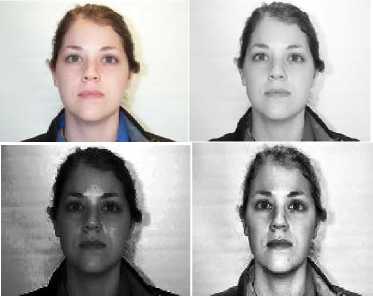
Fig. 1. RGB Image, Gray image, HE Image and AHE Image

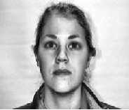
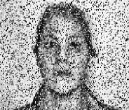
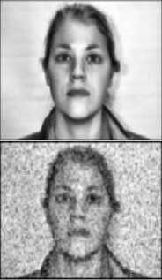
Fig. 2. AHE Image, GF image, Noisy Image and GF Image

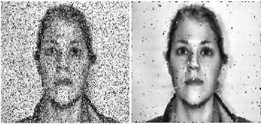
Fig. 3. Noisy Image and MF image

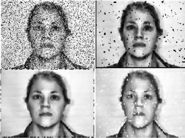
Fig. 4. 2DOF operated at different levels on noisy image

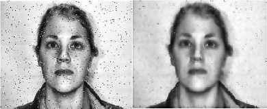
Fig. 5. Noisy image and WF image

3.    Pixel Difference Based Image Quality Measures (PDBIQM)

Pixel Difference Based Image Quality Measure (PDBIQM) [17] computes the error (difference) between the original image and distorted image. Numerous methods existing in literature uses PDBIQM. Let original image be denoted by I(i, j) and distorted image be denoted by K(i,j).

• A.    Mean Square Error (MSE)

MSE computes the mean square error between original image and distorted image. Low the error value, low will be the mean square error. The formula used for the MSE computation [18] is defined as.

1 ∑in=1∑jm=1[(I(i, j) -K(i, j)]2

• B.    Peak Signal To Noise Ratio (PSNR)

PSNR computes the ratio between peak power of signal image to noise corrupting the signal image. Higher the value of PSNR higher the clarity of the distorted image. Lower the value of PSNR lower the clarity of the distorted image. Formula for PSNR [28] is defined as.

10 log10 ( R2 ) MSE

R denotes maximum value (pixel) of input image. However in case of double precision floating point the value for R=1 and in case for 8-bit unsigned data types which are integers the value for R=255.

• C.    Signal To Noise Ratio (SNR)

SNR computes the ratio of max power in a signal image to the max noise in the signal image. The formula for SNR [29] is defined as.

[Max Power of Signal Image/Maximum Power of Noisy Image]

10log10(

)

• D.    Normalized Absolute Error (NAE)

The formula of NAE [30] is given in eq. 4. The numerator part shows the absolute difference within original and distorted image. The denominator part is used to find out absolute value of original Image. Numerator part should be as minimum as possible and denominator part is size of the original image. If numerator part is minimum then NAE is a close to zero, which is crucial for the experimental purpose.

∑ _i ⁿ ₌₁ ∑ _j ^m ₌₁ |I(i,j)-K(i,j)| ^∑ iⁿ=1 ^∑ j^m=1 ^|I(i,j)|

• E.    Structural Content (SC)

The SC [31] define the ratio of square of input image to the distorted image.

∑ iⁿ=1 ∑ jⁿ=1 I(i,j) ²

^∑ iⁿ=1 ^∑ jⁿ=1 ^{K(i,j) 2                                                               (5)}

• F.    Maximum Difference (MD)

The MD [31] generates the max absolute error between original image and distorted image.

Max |I(i, j) - K(i, j)|                                                  (6)

• G.    Average Difference (AD)

The AD [31] generates the Average Difference within the original image and distorted image.

1 ∑in=1∑jm=1(I(i, j) -K(i, j)

H. Laplacian Mean Square Error (LMSE)

The formula for LMSE is given in eq. 8. The value of LMSE should be as minimum as possible. Larger the LMSE value [19, 31] poorer the image quality.

∑ _i ⁿ ₌ ^-1 ₁ ∑ _j ^m ₌ ^- ₁ ¹ [L(I(i,j))-L(K(i,j))] ²

∑ _i ⁿ ₌₁ ∑ _j ^m ₌₁ L(I(i,j)) ²

Where L (I(i,j)) is the Laplacian Operator and whose value is L(I(i,j)=I(i+1,j)+I(i-1,j)+I(i,j+1)+I(i,j-1)-4I(i,j) In terms of matrix dimensions it is written as

0     10

1  -41

0    10

• I.    Normalized Cross Correlation (NCC)

The similarity between 2 images is measure by correlation function. In terms of the digital image processing NCC is the efficient technique for image assessment. The value of NCC range from -1 to +1. If this value is nearer to 1 then it is positive correlation and if closer to -1 then it is negative correlation. But both values produce better image assessment. However if value comes closer to 0 then it shows poorer image assessment. The formula of NCC [31, 32] is defined as.

∑ _i ⁿ ₌₁ ∑ _j ^m ₌₁ (I(i,j).K(i,j))

^∑ iⁿ=1 ^∑ j^m=1 ^{I(i,j) 2}

J. Image Fidelity (IF)

IF [31] is used to discriminate information loss between 2 images. The value of IF should be close to 1. 1 value indicate no difference between the original and distorted image, which means that numerator and denominators possesses 0 values. The numerator and denominator part should be close to 0. Formula for IF generation is defined as.

1-

∑ _i ⁿ ₌₁ ∑ _j ^m ₌₁ (I(i,j)-K(I,j) ²

∑ _i ⁿ ₌₁ ∑ _j ^m ₌₁ I(i,j) ²

As an example considering gray scale image and blurred image as shown in Fig. 6. After applying all measures on gray scale and blurred image, the results obtained are shown on Table 1. All testing is conducted in MATLAB R2008b environment.

Fig. 6. Gray image and blurred image (distorted)

Table 1. PDBIQM and its values

PDBIQM	Values
MSE	8.0873
PSNR	30.922
SNR	28.680
NAE	.0348
SC	1.0231
MD	.27-.57
AD	.0067
NCC	.9860
IF	.7290

4.    Edge Based Image Quality Measures (EBIQM)

To generate EBIQM, formula is described in [17], which is computed between the original image and distorted Image. In this section various edge detection techniques are discussed. Edges are very essential for feature extraction, which is then utilized for the classification. The major steps of edge detection are.

• a.    Image Enhancement (as discuss earlier) is used for improving image quality. There are many Image Enhancement techniques are described in [20, 21].

• b.    Detection of edges by using edge detection techniques are described in this section. Thresholding is used for proper edge detection. Numerous thresholds have been tested and the one which gives the best results will be taken as output. Several thresholding techniques are described in [32].

• c.    Final step is finding of exact location of edge pixels and this is achieved by image thinning [33].

In [34] numerous edge detection techniques are discussed. They are classified into 2 categories i.e. first order derivatives and second order derivatives. Some of the first order derivative techniques are Sobel [35], Prewitt [23] and Roberts [23]. First order derivative techniques are also known as gradient based techniques. In first order derivatives, the image is convolved with the respective mask and then edges are detected based on thresholding. The Robert operator uses 2x2 mask. These masks are the gradient masks in x and y directions. The mask is slide over original image and the output produced is the gradient image in x and y directions at point x and y denoted by J(x) and J(y). Ultimately J(x,y) is produced by performing square root of summation of the squares of gradient images. Eq. 11 delivers concept of J(x,y) formation, which is magnitude gradient.

1      0        01

0     -1       -10

J(x,y) = 7(J⁽x)) ² + (J⁽y)) ²

Sobel and Prewitt are 2 such operators which are mostly used in literature for the edge detection. Prewitt and Sobel both utilizes gradients in horizontal and vertical directions. The 3x3 mask used by Prewitt is defined as.

-1   0   1          -1   -1-1

-1   0  1         0   00

-1    0   1           1     11

Gradient at specific direction is also known as first derivative operator. Gradient in x direction is denoted by G(x) at points x and y, and gradient at y direction is denoted by G(y) at points x and y. In terms of pixel values of x and y matrix is defined as.

I(x - 1, y - 1) I(x,y - 1) I(x + 1, y - 1) I(x - 1, y)         I(x, y)      I(x + 1, y)

I(x-1, y+1)    I(x, y+1)   I(x+1, y+1)

According to Prewitt, the values of G(x) and G(y) at specific direction is given as.

G(x)=I(x+1,y-1)+I(x+1,y)+I(x+1,y+1)-[I(x-1,y-1)+I(x-1,y) +I(x- 1,y+1)]

and

G(y)=I(x-1,y+1)+I(x,y+1)+I(x+1,y+1)-[I(x-1,y-1)+I(x,y-1) +I(x+1,y-1))]

For producing the magnitude gradient, the masks are slide over the original image and the image evolves after is the gradient image in x and y directions, denoted by I(x) and I(y). Finally the magnitude of gradients (i.e. I(x,y)) is produced by performing the square root of summation of squares of gradients. Eq. 12 delivers concept of I(x,y).

I⁽x,y) = JCfto^+lCy))                              (12)

Similarly the magnitude gradient is computed in all 8 directions. The gradient formation in 8 directions gives clear information regarding the edges. The one which extracts more edges are considered for experimental purpose. One example of rotation gradient is described as: Suppose the 3x3 Prewitt mask is rotated to 450 then 3x3 mask looked like as defined below.

0   1   1         -1   -10

• - 1   0   1         -1    01

• - 1  -1   0         0    11

The gradient G(x) and G(y) at a 45 degree rotation is defined below.

G(x) =I(x,y-1)+I(x+1,y-1)+I(x+1,y)-[I(x,y+1)+I(x-1,y+1)+ I(x- 1,y)

and

G(y)=I(x+1,y)+I(x+1,y+1)+I(x,y+1)-[I(x-1,y-1)+I(x-1,y)+ I(x,y-1)

For producing the magnitude gradient, the masks are slide over original image and the image evolves after is the gradient image in directions x and y, signify by I(x) and I(y). Finally magnitude of gradients (i.e. I(x,y)) is produced by performing the square root of summation of squares of the gradients. Eq. 13 delivers concept of I(x,y).

I(x,y) = J(l(x))2 + (I(y))2

The mask used by sobel operator is defined as under.

• - 1   0   1              1   21

• -2  0  2        0  00

• -1   0   1         -1  -2-1

The gradients G(x) and G(y) at a specific direction is defined as

G(x)=I(x+1,y-1)+2I(x+1,y)+I(x+1,y+1)-[I(x-1,y-1)+2I(x- 1, y)+I(x-1,y+1)] and

G(y)= I(x-1,y+1)+2I(x,y+1)+I(x+1,y+1)-[I(x-1,y-1)+2I(x,y- 1)+I(x+1,y-1))]

For producing magnitude gradient, masks are slide over original image and image evolves after is gradient image in directions x and y, denoted by I(x) and I(y). Finally magnitude of the gradients (i.e. I(x,y)) is produced by performing square root of summation of squares of gradients. Eq. 14 delivers concept of I(x,y).

I(x,y) = J^Ito^+lCy))²                                (14)

The difference between the Prewitt and Sobel operators are in their mask values. The middle value used by Sobel is 2 and that of Prewitt is 1. By using different threshold value the edges are extracted. The threshold value should be as minimum as possible. If I(x,y)>threshold then more edges are detected in contrast threshold>I(x,y). The direction formula in 8 directions (i.e. 450, 900, 1350, 1800, 2250, 2700, 3150, and 3600) is portrayed in eq. 15. The direction which gives the best edge response is taken as output.

Theta = tan-(y)(15)

In second order derivatives there is a zero crossing which gives the edge direction. One of second order derivatives is Laplace of Gaussians (LOG) [23] [36]. The LOG considers the pixel dimension in x and y directions. The first order derivative in x and y directions are defined as.

∆1=I(x, y)-I(x-1, y)(16)

∆2=I(x+1, y)-I(x, y)(17)

∆3=I(x, y+1)-I(x, y)(18)

∆4=I(x, y)-I(x, y-1)(19)

Difference between ∆1 and ∆2 is second derivative in x directionas shown in eq. 20.

£-=A2 - Al = I(x + 1, y) + I(x - 1, y) - 2I(x, y)

Difference between ∆3 and ∆4 is second derivative in y direction as shown in eq. 21.

§=A3 - A4 = I(x, y+1) + I(x, y-1) - 2I(x, y)(21)

If both derivatives are added then output is given in Eq. 22

bI +b- =I(x+1, y)+I(x - 1, y)+I(x, y+ 1)+I(x, y-1)- 4I(x, y)

To represent this output in matrix dimensions is expressed as

0    10

• 1 —41

0    10

This operator is known as Discrete Laplacian Operator (DLO) [24]. If this operator is deployed on original image then edge locations are given by the zero crossing. But if there is a noise persistence then it will be highlighted after deploying DLO. So it becomes difficult to distinguish genuine edges. Therefore in noise this operator is not useful. To make it useful the LOG [37] operator should be employed. The gaussian and LOG formula are defined in eq. 23 and eq. 24.

g (x,y)= 2n_ _ e_Xp(^— x^+z ^- )                                   (23)

LOG = c [1 — (^)exp (— ^)]                        (24)

The gaussian filter is used for the image smoothing and Laplace is conducted further to extract the edges. Therefore LOG is effectively used for the image matching. Another edge detection technique is given by the John Canny [38], which is known as the Canny edge detection. The Canny edge detection comprise of 5 stages.

• a.    In first step the image smoothening is performed for noise removal. To accomplish this gaussian filter is used.

• b.    Then gradients are computed (by Sobel) in x and y directions which is followed by the computation of magnitude gradient.

• c.    Then gradient value is formed in 8 directions. The direction which gives the best edge strength is considered and lower one is rejected.

• d.    Further threshold is used for detecting edges. In Canny two threshold are used, one for detecting weak edges and one for detecting strong edges. Edge pixels bigger then high threshold are considered strong. Edge pixels lower then low threshold are rejected. Edge pixels lie between the lower and high threshold values are considered weak edges.

• e.    Finally edge tracking is done by hysteresis. Strong edges are shown by true edges. Some weak edges can persist due to noise.

The major challenge in edge detection is the amount of sigma values to be used. The sigma value detects the number of edges using distinct values. As an example the gray scale image is considered and after applying first order derivative operators the output images are shown in Fig. 7. Edge detection analysis is performed on image in [27] and all testing is done in MATLAB R2008b by various functions. Figure 7 shows that there is very less variation between the Sobel and Prewitt edge detection techniques, but still there are some places where Sobel edge detection is superior than the Prewitt edge detection. Another difficult task (in edge detection) is setting of threshold therefore same threshold is chosen for Prewitt and Sobel operator and different threshold is chosen for Robert operator. Fig. 8 shows result of second order derivatives which include Canny edge detection and LOG edge detection. Canny produces more edges as compare to others. Therefore Canny edge detection is best. Fig. 9 shows the result of Canny edge detection on different sigma values. In simpler words the Canny edge detection algorithm is far better than the other algorithm. Figure clearly shows as value of sigma increases edge detection becomes lower and if value of sigma decreases edge detection becomes higher. So a great care should be taken in choosing sigma because very low sigma value also produces false results. The value of sigma’s which are used in this analysis are (.7, 1, 1.5, 2 and 2.5). Fig. 10 shows 5 variations of Sobel edge detection at different thresholds.

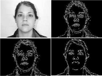
Fig. 7. Gray image, Sobel image, Prewitt image and Roberts’s image

Fig. 8. Gray image, Canny image and LOG image

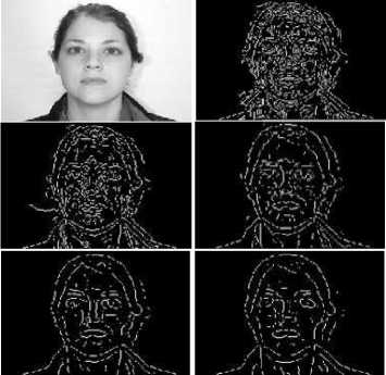
Fig. 9. Canny results on 5 sigma values (.7, 1, 1.5, 2, 2.5)

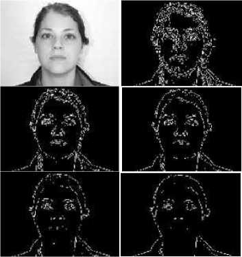
Fig. 10. Sobel images at different threshold values (.020, .040, .060, .080, .1)

5.    Corner based Image Quality Measures (CBIQM)

To build Corner Based Image Quality Measures (CBIQM) the formula as defined in [17] and is computed between original image and distorted image. This section describes various Corner Detection Techniques. Corners are also essential parts for feature extraction. If Corners are detected accurately then it benefits feature extraction and image matching. The Corner detection is classified into 2 categories: Interest Point Detectors and Contour Based Detectors. In Interest Point Detectors, corner is analyzed from the image gray values. There were numerous Interest Point Detectors persist in literature. Some are discussed in this section and rest are discussed in Table 2. The most important Interest Point Detector is given by Harris [39, 40]. The Harris detector is based on the matrix associated to function based on auto-correlation. Formula is defined as.

R = det (M) - k(trace M)2                                   (25)

k is constant, vary between (0.4-0.6). R completely depends on eigen values of M. If eigen values are large then detected point M is 2x2 matrix which is defined as.

⁽I x ⁽x,y^{)) 2}      I x ⁽x^,y^)I y ⁽x,y⁾

^X,y      I x ⁽x,y⁾I y ⁽x,y^{)     (}I y ⁽x,y^{)) 2}   J

I_x(x, y) and I_y(x, y) are image gradients in directions x and y at points (x,y). These are computed by performing the convolution between image and the mask. Square of the image gradients are convolved with the gaussian function to minimize the noise. (I x (x, y))² , (I y (x, y))² are square of the image gradients. g(x,y) is Gaussian function. I x (x, y)I y (x, y) is the convolution between gaussian function and multiplication of image gradients (in x and y directions). This is standard Harris operator but there are some drawbacks in this operator as suggested by Schmid [40]. Schimid [40] experiments suggest that the results of Harris detector are not satisfactory. In improved version of Harris the performance increases rapidly. This is due to the different mask (-1 -2 0 1 2) utilization. The improved version produces much better outcomes in rotation, scale, illumination, viewpoint and noise transformations. The other crucial interest point detector is known as Smallest Univalue Segment Assimilating Nucleus (SUSAN), given by Smith et al. [41]. SUSAN operator works on image edges and corner detection consists of a various circular masks which is different from earlier masks. The center portion of each mask is known as nucleus, which is compared with other pixels within the mask. If the difference between other pixels (within the mask) and nucleus coordinates is less than or equal to the threshold (value of that mask) then edge point is detected. The threshold values are used for detecting the noise. Likewise similar operation is performed on each mask. When points are detected (on the whole template) then that value is compared with geometrical threshold. If value is less than geometric threshold then corner is detected. Advantage of SUSAN operator is threshold utilization in edge and corner detection which is crucial in noise removal. The contour based detectors are defined in Table 2. In Table 2 numerous interest point detectors and contour based detectors are discussed. These are developed for different applications. The total count of such work are 7. CBIQM is the second sub-objective of the research conducted in the presented work.

Table 2. CBIQM work

Ref.	Other authors work
[42]	Moravec detection was based on autocorrelation function. The Moravec concept is used for calculating the gray difference between the window and windows shifted in 8 directions. If minimum value (of these differences) is greater than chosen threshold then point is detected.
[43]	Kitchen and Rosenfeld proposed the corner detection in which gradient direction change is computed on edge contours. Then it is multiplied by gradient magnitude for achieving the corner detection.
[44]	Beaudet detection was based on second order derivatives of image signal.
[45,46]	In this work the detection is based on autocorrelation function matrix. First the original image is converted into blurred image and then derivatives are computed which is then summed over a Gaussian function. Forstner takes 2 eigen values for defining axes of error ellipse.
[47]	Tomasi and Kanade worked in tracking area, based on autocorrelation matrix known as Tomasi and Kanade operator. Depending on the eigen values of correlation matrix the feature point is detected.
[48]	Heitger proposed a method based on biological visual system. Gabor filters are used to extract 1D directional characteristics. Then first and second order derivatives are computed to obtain 1D and 2D characteristics.
[49]	Cooper proposed a method in which contour directions are measured and then image difference is calculated on contour directions. Noise factors are also ponder, which makes easier to find edge point in contour directions.

6.    Conclusion

Image Enhancement is the crucial phase of the particular application. These Enhancement Techniques becomes essential when there is every possibility of image degradation due to the uncontrolled variations. These variations are categorized into light, emotion, noise, pose, blur and corruption. The enhanced images provide much better images from which the feature extraction is performed more effectively. Therefore the two major objectives of the proposed work are aligned in two phases . First phase of this paper discuss the Enhancement Techniques for improving the image intensity. Second phase provide detailed elaboration of various FRBIQM. The FRBIQM is further categorized into PDBIQM, EDBIQM and CDBIQM. The first image quality measure employs different techniques to evaluate performance between original image and distorted images. Second image quality measure deploy various Edge Detection Techniques, which are essential for increasing the robustness (in feature extraction) and third image quality measure discuss various Corner Based Detection Techniques, which are essential for enhancing the robustness (in feature extraction). All these techniques are discussed with their examples. This paper provides brief survey of IET and FRBIQM. The significance and the value of the proposed work are to select the best image enhancement techniques and image quality measures among all (described ones) for features extraction. The one which gives the best results will be used for feature extraction.