Analytical Model for Wireless Channel of Vehicle-to-Vehicle Communications

Published Online July 2017 in MECS DOI: 10.5815/ijwmt.2017.04.05

V2V communication systems are ad hoc based that connect vehicles that are highly dynamic, so the path loss must be considered to analyze the interference and scalability. Path loss depends on the type of environment such as highway, rural, urban, and suburban. The signal that is travel from the transmitter to the receiver antenna through channel suffers from attenuation and scattering due to the environment and distance between them [2]. Power delay profile (pdp) is the distribution of signal power of the received signal after traveling into a multipath channel as a function of the propagation delay [6]. The delay spread is a type of distortion which effects on the transmitted signal and lead to arriving it at different times to the destination. The signal usually takes a multi path with different angles, so the angles of the received signal are different. Maximum access delay is the difference between the moment of arriving of the first multipath component (usually the line of side path) and the last multipath component. The root mean square (RMS) delay spread is the square root of the second moment of the power delay profile [7]. Authors in [8] analyzed channel with introducing a model for a channel between vehicles that are moving in the same direction and operating at 2.4 GHz and in [9] for 5.9GHz band. Results of path loss measurement, pdp and RMS delay spread for vehicles driving in opposite directions are evaluated in [2] at 5.2 GHz. Basic physical layer concepts of channel mode (i.e. path loss, Shadowing and multipath power delay profile) are modeled in [3]. This paper introduces analytical analyses for the system taking into account influence multi natural obstacles which may face traveling signals between communicating vehicles. This paper considering many scenarios for the state of the vehicles, such as stopping moving cases with existing some obstacles that may face traveling exchanged signals between vehicles. The direction of the vehicles moving through Doppler Effect is also considered. The achieved results show that the path loss increases with increase the distance between the transmitter and receiver. The location of obstacles also effects on path loss. A power of transmitted signal is decreased with increases distance (i.e. increase excess delay) between the transmitter and the receiver.

The remainder of this paper is organized as follows: Section 2 illustrates wireless channel model between V2V. Section 3 shows the results for path loss, pdp and RMS delay spread. Section 4 is the conclusions of this paper.

• 2.    Wireless Channel Model

Wireless channel model is a mathematical model to analyze the carrier's medium for the signals that travels from the transmitter to the receiver. Since the connection is wireless, so the state of the channel is frequently changed. For this the analysis of the wireless channel mode is difficult since there are many obstacles between transmitter and receiver particularly in urban areas, therefore the transmitted signal is suffering to scattering, reflection, diffraction shadowing. These compose fading in the transmitted signals. There are two types of fading: large scale fading and small scale fading. The average signal power attenuation and path loss due to motion in the long distance are called the large-scale fading, in which the path loss and shadowing are takes into account. Small-scale fading is the change in the signal amplitude and phase after propagating in short distances.

Consider a simple sketch shown in Fig. 1. The received signal y(t) is the response to the transmitted signal x(t). After passing through the wireless channel with impulse response h(t,T) the received signal is:

x(t)

Channel h(t, t)

y(t)

Fig.1. Linear channel y (t) = x (t) * h (t, т) + n

where n is additive white Gaussian noise with zero mean and variance σ2. The * sign is the convolution expression. The time-varying frequency response is dependent on attenuation and propagation delay which may be expressed as [10]:

L - 1

H ( f , t ) = ^ a i ( t ) e - ^{j2 n f T}- ( t ⁾

i = 0

a i (t) is the attenuation in the ith path between the transmitter and receiver and τ i (t) is the propagation delay at time t for the ith path. Wireless channel between V2V connections are effected by:

• 2.1.    Free space

Free space is the simplest model, when there is no obstacle between the Tx and Rx the transmitted signal is propagated along a straight line. In this case, the attenuation and delay of the transmitted signal due to passing through the free space is:

x              r + vt <  9

a ( t ) =       ,       т ( t ) = -0    -—                                                    ⁽³⁾

• r ₀ + vt                c    2 n j

• 2.2.    Reflection

• 2.3.    Scattering

where Ɵ is the transmitted angle, r o is the location of the receive antenna and c is the speed of the light.

The signal may be reflected from walls, ground, or some objects, which make the signals pass in the long distance until be received by the Rx. In this case, the attenuation and delay is given by hit,

\ x                     2 d - r - vt <  9

,             т ( t ) =        ⁰       -

2 d - r ₀ - vt                      c       2. n f

The transmitted signal is travel through the medium to reach the destination. The carrier's medium may be consist of one or multi obstacles (such as trees, building, cars…) between the transmitter and the receiver. So this signal may be interfering on these obstacles that are caused to decrease the power of this signal and scattering the rest.

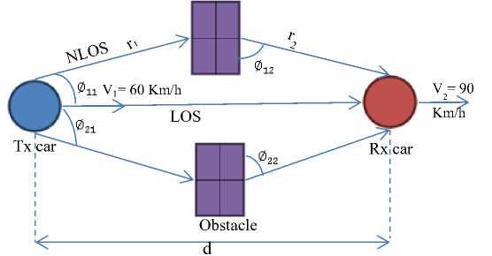
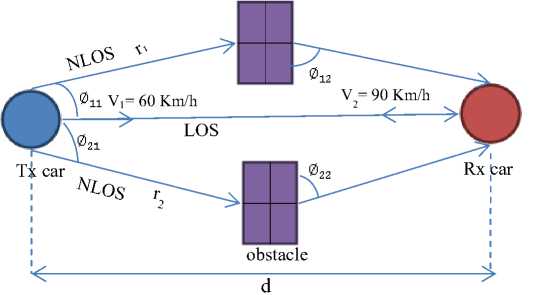
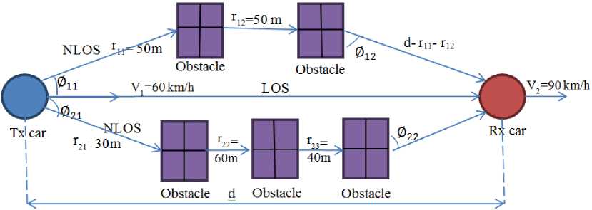
Consider the case when one's obstacle between the Tx and Rx the obstacle is located away from the Tx and Rx in distance (r1 and r2) m, respectively, with moving velocity of Tx and Rx car is v1 and v2 km/h, respectively, as shown in Fig. 2. Therefore the attenuation and delay may be calculated from [11]:

x r + vxt

T i ( t ) = r t c

—

< 6 ii

2f

(5.a)

a

^T 1 ( t ) =

—

c

2П

(5.b)

(5.c)

Power loss due to the path, Path loss (PL), may be evaluated from the received power (Pr), which is the magnitude square of the channel coefficient:

Then

P _ = P _

LdB    tdBm

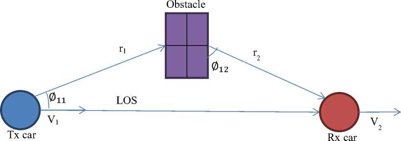
Fig.2. LOS and NLOS paths between the Tx and Rx cars.

where Pt is the transmitted power. Here, it taken as 27 dBm [2]. Power delay profile (pdp) is a center for any analysis or simulation for delay spread [12]. It is the string of the received signal after passing through multipath. Pdp is

Mean excess delay is the first moment of the power delay profile, is given by:

γ1 =

a2τ ii

i

i

To estimate the performance of the systems it is essential to find the spread of the multipath delay. It can be measured through the total delay span in the transmitter which is also called the excess delay spread. It is expressed by the RMS delay spread. RMS delay spread shows the special values among all values and error probability due to delay dispersion. RMS delay spread is the second moment of the pdp, it may be expressed by [6]:

σRMS = V γ1 -γ22

where

∑ 22 a ² τ ² ii

^γ 2 ⁼

i

∑ a i ²

i

• 3.    Simulation Results

Considering a sinusoidal signal is transmitted from transmitter side and it is suffering from attenuation, delay, and distortion due to the distance and obstacles between the Tx and Rx sides. Figure 3 illustrate the received signal after passing through the medium that content two obstacles in two NLOS paths away from the transmitter in 50m, and the distances between the Tx and Rx are 100m,200m, and 350m, respectively.

The path loss, pdp and RMS delay spread for 5.2 GHZ carrier frequency will be presented for different cases:

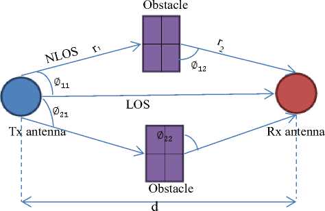
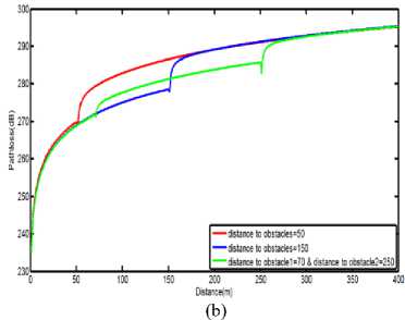
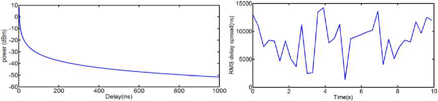
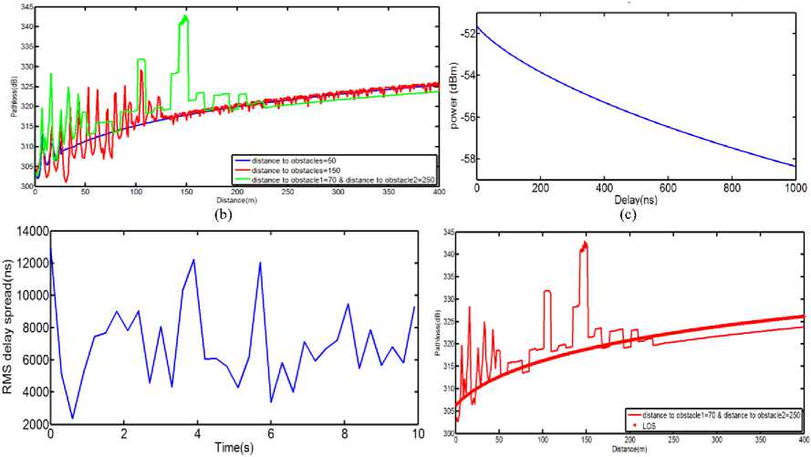
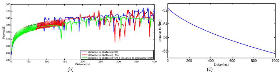
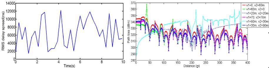
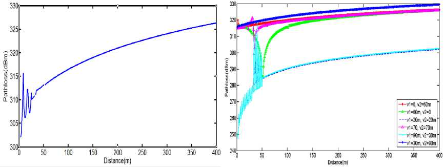
Case 1 . The distance between the Tx antenna and Rx antenna (d) is changed from 1 to 400 m. Three propagation paths are considered. One path is a line of side (LOS) and the two other paths are no line of side (NLOS) with (Ɵ 11 , Ɵ 12 ) and (Ɵ 21 , Ɵ 22 ) transmits angles, respectively. The distance from Tx antenna to an obstacle in the upper NLOS is r 1 and r 2 is for the down NLOS, as depicted in Fig. 4 (a). Fig. 4 (b) illustrates the path loss as a function of the distance between the transmitter and receiver. The results in red for the d = 1-400 m, r 1 = r 2 = 50 m, Ɵ 11 = 30^o, Ɵ 12 = -60^o, Ɵ 21 = -45^o and Ɵ 22 = 60^o. The path loss increases in distance 50m because of the r 1 =r 2 =50 m. When r 1 = r 2 = 150 m the result in blue, the path loss increases and become more strong beyond 150 m. When r 1 = 70 m and r 2 = 250 m the result in green shows that a path loss increases in 70 m and 250 m, i.e. that due to the location of these obstacles and long distance effects on path loss. When the r 1 = r 2 = 50 m the pdp is illustrated in Fig. 4 (c) as a function of the excess delay. The power of the signal after passing in multipath decreases with increases the delay because of the distance between the Tx and Rx and noise increases. Fig. 4 (d) shows the RMS delay spread as a function to time dispersion. This is the performance of the wireless channel that is shown in Fig. 4 (a). This result is oscillator due to change in the received power in different time.

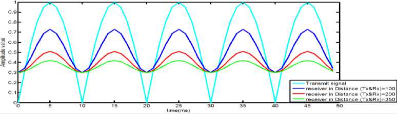
Fig.3. Transmit and receive signal

(c)

(d)

Fig.4. (a) carrier's medium between Tx and Rx antenna; (b) path loss as a function of distance,;(c) pdp with respect to excess delay and (d) RMS delay spread with time.

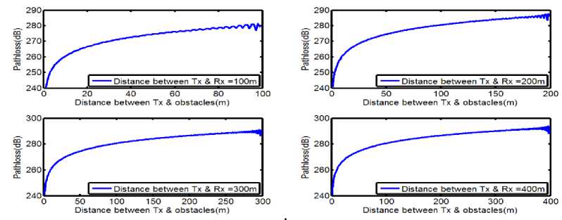
Case 2 : When the distance between Tx and Rx antenna (d) is fixed. Four distances are considered; 100, 200, 300, and 400 m. The distance between the transmitter and obstacle (r 1 , r 2 ) is moving from Tx to Rx antenna, as shown in Fig. 4 (a). When obstacles are near from the Tx the path loss is low and increases when obstacles are moving away from the Tx toward the Rx. Whenever the distance between the Tx and Rx increases, the path loss increases, as illustrate in Fig. 5.

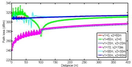
Case 3 : Transmit and receive cars are in moving in the same direction with different velocities of the Tx and Rx cars; 60 and 90 km/h. So the distance between the Tx and Rx (d) is changed according to due to values of the v 1 and v 2 , as shown in Fig. 6 (a). The overall path loss between vehicles is given in Fig. 6 (b). The path loss becomes smooth when the distance is near 50 m due to the location of the obstacles which are close to the Tx when the separation is getting larger. The attenuation is caused by the obstacles lead to decrease the strength of the signal. As shown in Fig. 6 (b). The results in green is suffering from the distortion because the attenuation in the signal that is caused by distance and obstacles. Due to r₁ = 70 m and r₂ = 250 m, the shape of path loss is changing after 70 m and 250 m.

When the distance between the Tx and Rx increases leads to increase the delay to excess the signal to the receiver side and decrease the signal power as shown in Fig. 6 (c). RMS delay spread as a function of the time is illustrated in Fig. 6 (d) that is shown the performance of channel between V2V.

When r 1 =70m and r 2 =250m the signal may be pass in the direct path between Tx and Rx car (LOS) that is not found obstacles along this path i.e. only distance between Tx and Rx is an effect on the power of the transmit signal. While when transmit signal is divided into three paths that are shown in part (a) of this Figure, the power of the transmit signal is suffering to more attenuation due to the distance and obstacles between Tx and Rx as shown in Fig. 6 (e). The communication cars velocity has an effect on the path loss as clear in part (f) from Fig. 6. The velocity of the transmitting car has a great effect on path loss from receiver's car velocity. When a communication cars are movies in the same velocity, there is no a significant impact on the path loss.

Obstacle

(a)

(e)

(d)

(f)

Fig.6. (a) Channel, (b) path loss as a function of distance, (c) pdp for LOS path, (d) RMS delay spread with respect to time, (e) path loss of the signal that is passes only in LOS path and on three paths (LOS and 2 NLOS paths) and (f) path loss for different velocities of the Tx and Rx car.

Case 4 : Tx & Rx cars are moving in opposite directions with different velocities as depicted in Fig. 7 (a). The path loss of this case is shown in Fig. 7 (b). It is clear that the direction of moving has a strong affected on the path loss due to Doppler Effect. When the Tx and Rx cars are moving toward each other the frequency increases. The amplitude and delay of the transmitted signal are changed with frequency. It is obvious that the path loss is smoother when r 1 ≠ r 2 (results in green). Pdp and RMS delay spread for LOS path between vehicles moving in opposite direction as shown in part (c, d) for Fig. 7.

The effect of a change in velocity on path loss is illustrated in part (e) in Fig. 7. Transmitter's velocity have a great effect on path loss from receiver car.

obstacle

(a)

(d)

(e)

Fig.7. (a) Channel, (b) path loss, (c, d) pdp and RMS delay spread for LOS path and (e) path loss for different velocities.

Case 5 : Existing obstacles between transmit and receive cars. Fig. 8 (a) shows existing multiple obstacles between the Tx and Rx cars. The first obstacle in the upper of the NLOS path is away from Tx car in 50 m and two obstacles in 100 m. The down NLOS path there is three obstacles away from Tx in 30, 90 and 130 m, respectively. Path loss that is shown in Fig. 8 (b) for the medium in part (a), increases with increasing the distance between the Tx and Rx. The power of a transmit signal is less after passing from obstacles, at the receiver side, the signals received from three paths are constructive add.

Fig. 8 (c) shows the effect of change velocity of Tx and Rx car on path loss. When the communication cars move in same slow velocity, the path loss is less than path loss when cars move in same fast velocity.

(a)

(b)

(c)

Fig.8. (a) medium for multiply obstacles, (b) path loss as a function of distance and (c) path loss for different velocities.

• 5.    Conclusions

This paper presents a model for evaluation of a V2V channel at 5.2 GHz with different scenarios. The analyses and achieved results show that increasing the distance between the communicating vehicles leads to increasing the path loss with decreases the received power. Location of the obstacles with respect to the communication vehicles also affected on the overall path loss value. The obstacles are near to the transmitter or receiver car more effect on the quality of the received signals. The direction of motion is considered for the same or obesity direction, therefore they effect in path loss, pdp, and RMS delay spread.

Delay between transmit and receive signal in another side affected on the power delay profile that is lead to decreases it. RMS delay spread also change with increase arrive time of the received signal.