Anchor-Free Yolov8 for Robust Underwater Debris Detection and Classification

Densely populated cities and industrial development have resulted in massive amounts of domestic and industrial garbage, which majorly gets dumped in the ocean. Today, the sea coast, seabed, open sea, and deep sea are heavily dumped with man-made debris. Garbage is on the sea coast, floating on the sea, and also in the deep sea. This marine debris is harmful to the marine life and it also contaminates seawater. Oceans and aquatic ecosystems around the globe play a crucial role. The micro plastics, formed by dumping plastic, enter the food chain and pose harmful threats to humans and the ecosystem. The widespread issue of underwater debris continues to put these ecosystems at risk.

The garbage that flows into the sea is continuously eroded by the water and pressure, which results in changes in the size and shape of the objects. It is difficult to find and categorize underwater debris traditionally, as it requires extensive manual image processing and human divers.

For the task of removing marine garbage, vision robots or, submersibles or, autonomous underwater vehicles (AUVs) are used. AUVs use object detectors and locators to find the debris. The task of removing marine garbage has two parts: detecting and removing the marine debris.

This project aims at using deep learning methods for detecting underwater debris. These deep learning models can automatically detect and classify underwater debris, mitigating the limitations of manual techniques. It also enhances efficiency and accuracy. Moreover, these can adapt to diverse environmental conditions and thus provide an approach to this multifaceted problem.

The problem of Debris Detection can be categorized into two types: Surface Marine Debris Detection [1, 2, 3, 4] and Underwater Debris Detection [5, 6]. In the case of surface marine debris detection, various machine learning and deep learning techniques have achieved good performance. However, the problem of underwater debris detection is challenging and is studied very little. It is addressed by very few researchers. As compared to the surface debris detection, the underwater debris detection problem has more complexities. Major challenges for deep-sea marine debris detection are: due to the water environment’s weak light, marine debris is deformed, eroded, and blocked. In the detection task, a major disturbance may be created by the real marine life and environment: fish, animals, rocks, algae, marine flora, etc. Another major challenge is the real dataset availability for the task of underwater debris detection. Capturing data This work is open access and licensed under the Creative Commons CC BY 4.0 License. Volume 14 (2022), Issue 6 in the deep sea requires huge manpower and various resources such as professionals with deep diving equipment, high precision cameras for recording real underwater debris images and video recording. Therefore, the task of underwater debris detection is challenging. Some of the complexities are listed here:

Real Deep-Sea Debris Dataset Availability: The task of data collection is challenging. Data need to be captured under seawater at the maximum depth with high-definition cameras.

Uncertainties in the dataset: Due to lack of sunlight in deep sea, underwater animals and plants, rocks, algae, and marine flora and fauna.

Erosion of Deep Sea Debris: Erosion of debris in deep-sea results in changes in shape, size, and texture of underwater debris.

Object Detection Methods: Natural object detection methods cannot be applied to underwater debris detection problems due to underwater environment, weak light, and erosion of debris due to seawater.

Various object detection and classification methods based on deep convolution neural network models [7] such as VGG16 [8], ResNet50[9], MobileNetV2[10], InceptionResNetV2[11], FasterRCNN[12], SSD [13], YOLOV3[14], YOLOV4[15], YOLOV5 [16], EfficientDet-D0[17] have been applied and experimented with the underwater debris detection problem. Research carried out for underwater debris detection has two types of detection networks:

Two stage Network: Two stages in a two stage network are, Identifying the position of the object and classifying/detecting the objects. For example, models like Faster R-CNN, Mask R-CNN, and Cascade R-CNN. Two stage networks have very good detection accuracy but the detection speed is compromised.

One stage network: In case of one stage network, region proposal stage is eliminated. It directly begins from the detection stage. Example models include YOLO, SSD, and RetinaNet. One stage detection networks have faster inference/detection speed but the accuracy is compromised.

In the research proposed by various researchers, researchers have worked on seven debris categories: plastics, fishing nets, cloth, metal, rubber, natural debris, and glass. Majority of the Debris Detection approaches focus on plastics and water bottles. However, fishing nets cause maximum threat and are responsible for the greatest percentage of plastic in the ocean.

2.    Literature Review 2.1.    One Stage Underwater Debris Detection using ResNet50-YOLOV3

Xue et al.[18] have proposed one stage detection network with ResNet50-YOLOV3 for underwater debris detection. In this one stage network, the structure is divided into two parts: ResNet50 is the backbone. It works as a feature extractor. YOLOV3 works as the feature detector. The accuracy and speed of the one stage detection network are improved with the use of ResNet50-YOLOV3.

Table 1. Objects in JAMSTEC[19] Dataset

SN	Type of Object	Count
1	Plastic	3768
2	cloth	2518
3	Natural Debris	2268
4	Fishing net and Rope	2003
5	Metal	1999
6	Rubber	1285
7	Glass	1161
8	Total Number of Objects	15002

Dataset used is Japan Agency for Marine-Earth Science and Technology (JAMSTEC). JAMSTEC has prepared the deepsea debris dataset [19] containing real underwater debris images and videos. In this work, the required dataset is generated by extracting appropriate frames from JAMSTEC[19] dataset videos and are combined with images. The dataset has 10000 3D images with dimensions 480 × 320. Seven debris categories are covered in the dataset. Categories are: fishing net and rope, cloth, rubber, glass, natural debris, plastic, and metal. As shown in table 1, the dataset contains 15002 objects in 10000 images.

Network Architecture is as follows: The input size of the network is 416 × 416. The architecture is divided into two parts: (1) Feature Extractor - ResNet50 (2) Feature Detector - YOLOV3.

Feature Extractor - ResNet50 [9] Network can be defined as: 7 × 7 convolution and 3 × 3 max pooling for preliminary processing, ResNet Block1: 3 ResBlocks, ResNet Block2: 4 ResBlocks, ResNet Block3: 6 ResBlocks, ResNet Block4: 3

ResBlocks. Feature map of 13 × 13 × 2048, YOLOV3

Feature Detector - YOLOV3 [14]: With an input of 416 x 416, it makes detections on scales 13 x 13, 26 x 26, and 52 x 52.

Baseline Methods Used for Comparison are: SSD [13] and Faster R-CNN [12] detectors are used as the baseline for comparison with the YOLOV3 detector. Three classic classification networks ResNet50, VGG16 [8], and MobileNetV2 [10] are used as baseline for comparison with feature extractor. As shown in table 2, total of 8 comparative methods are used for the performance analysis of ResNet50-YOLOV3.

Table 2. Baseline Methods for Performance Analysis of ResNet50-YOLOV3

Sr.No	Feature Extractor	Feature Detector
1	VGG16	FasterR-CNN
2	MobileNetV2	FasterR-CNN
3	ResNet50	FasterR-CNN
4	VGG16	SSD
5	MobileNetV2	SSD
6	ResNet50	SSD
7	VGG16	YOLOV3
8	MobileNetV2	YOLOV3

Required Experimental Environment: Operating System: Microsoft Windows 10, Processor: Intel(R) Xeon(R) W2133 CPU at 3.60 GHz, Graphics Card: GeForce GTX 1080Ti GPU with a capacity of 11 G.

• 2.2.    One Stage Underwater Debris Detection using Shuffle-Xception

Aim of the work carried out by Xue et al.[20] is to evaluate the performance of a convolution neural network for underwater debris detection problem. It aims to determine if CNN can efficiently and accurately identify underwater debris. In this work, the Hybrid Shuffle-Xception network is used to identify the underwater debris.

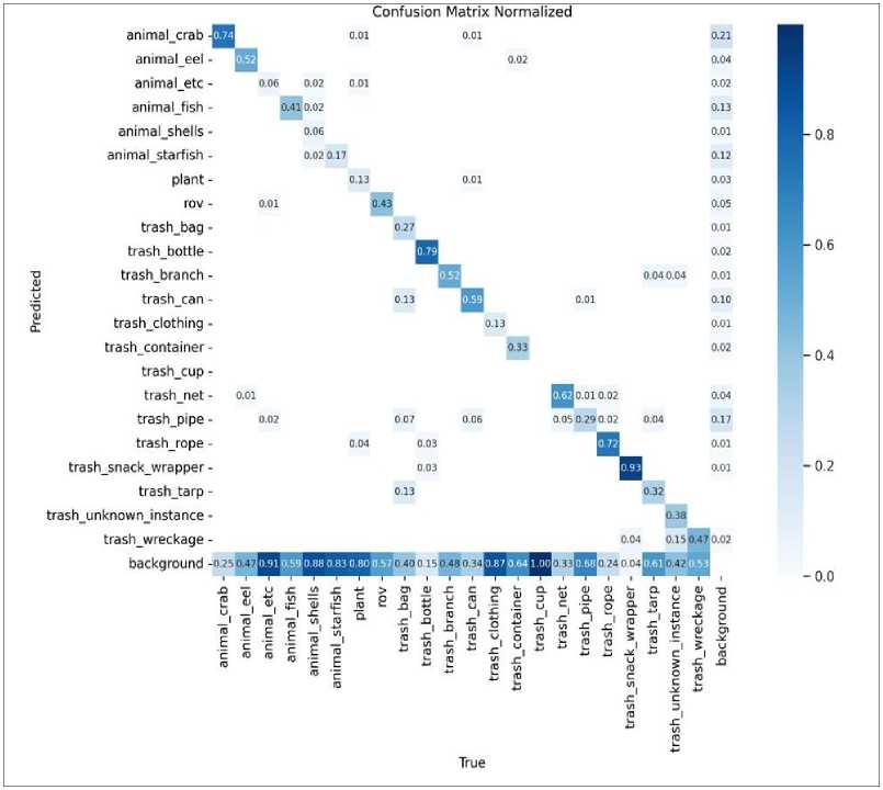
Fig. 1. YOLOV8 Confusion Matrix with Instance Version

Dataset used in this work is DDI. A real deep sea debris dataset called as DDI is constructed from the Japan Agency for Marine-Earth Science and Technology (JAMSTEC) dataset [19]. DDI dataset has 13914 deep sea debris images of seven categories of debris including: “plastic, fishing net, rope, metal, cloth, rubber, glass, and natural debris”. Every image has only one type of garbage. In this implementation, the DDI dataset is divided into three sets: Training set: 70%, Validation Set: 15%, and Test Set: 15%.

Network Architecture is divided into three stages. (1) Entry Stage, where Ordinary convolution is performed twice. Shuffle-Xception(SX) unit is performed six times. Each two SX units form one group. Hence three groups are formed. (2) Middle Stage where 24 Shuffle-Xception(SX) units are used. A sequence of three units of SX units forms one group. This forms eight groups in total. Exit Stage where Four SX units are performed. There is one shortcut connection, Global average pooling (GAP), and One fully connected (dense) layer using the Softmax activation function.

Baseline Methods Used for Comparison: Five convolution neural networks (CNNs) frameworks are used for comparative performance evaluation. These five CNN frameworks are the classic deep learning networks. These are used in computer vision(CV) classification tasks.

ф

animal eel - anima l_etc - animal fish - animal shells - anima!_starfish - trash fabric - trash_fishing_gear - trash metal - trash_paper - trashplastic trash_rubber - trash wood -

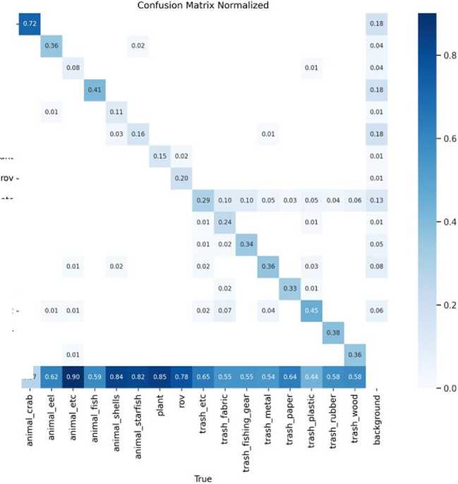
Fig. 2. YOLOV8 Confusion Matrix with Material Version

plant -

trash_etc -

background - 0.27

ResNetV2- 34 [21]: has 34 layers where the batch normalization and ReLU activation precede the convolution layers.

ResNetV2- 152 [21]: has 152 layers where the batch normalization and ReLU activation precede the convolution layers.

MobileNet [22]: It uses depthwise separable convolution instead of ordinary convolution.

LeNet [23]: The sigmoid function used in LeNet is replaced with the ReLU activation function and the subsampling is replaced with the max pooling.

Required Experimental Environment: Operating System: Microsoft Windows 10, Processor: Intel(R) Xeon(R) W-2133 CPU at 3.60 GHz, Graphics Card: GeForce GTX 1080Ti GPU, RAM: 31.7 GB RAM

• 2.3.    One Stage Underwater Debris Detection using YOLOV4

Work proposed by Zhou et al. [24] for deep sea debris detection is using YoloV4. The algorithm proposed in this work has two parts: backbone-feature extraction and feature fusion . Major achievements of this work are: improved accuracy and reduced size of the network model.

Dataset: TrashCan dataset [25] is used in this implementation. TrashCan dataset images are obtained from Japan Agency for Marine-Earth Science and Technology (JAMSTEC) dataset [19]. TrashCan has 7212 annotated RGB images. TrashCan is labelled with two versions.:

TrashCan Instance: It has 22 object categories: “marine trash, rov- man made, animals, plants, bag, container, etc.”.

TrashCan Material: It has 16 object categories such as “trash, rov, bio, unknown, metal, and plastic”.

Network Architecture: Model architecture is divided into two parts. YOLOV4 uses backbone and feature fusion models.: “ECA DO Conv CSPDarknet53”: It is called as Backbone. This is a feature extraction module used for extraction of “depth semantic features”.

“DPMs PixelShuffle PANET”: It is a Feature fusion module, used for improving detection ability.

Baseline Methods Used for Comparison: YOLOTrashCan performance is evaluated and compared with five baseline object detection networks including, SSD with VGG16, EfficientDet- D0 with Efficientnet-B0, Hong Methods, YOLOV3 with Darknet53, YOLOV4 with CSPDarknet53. Table 3 describes the baseline methods.

Table 3. Baseline Methods for Performance Analysis of YOLOTrashcan

Model	Backbone	Resolution
SSD [13]	VGG16	300 X 300
Efficientdet-D0 [17]	Efficientnet-B0	512 X 512
Hong-Faster RCNN [25]	ResneXt 101 32 8d	800 X 1333
YOLOV3[14]	Darknet53	416 X 416
YOLOV4[15]	CSPDarkNet53	416 X 416

Required Experimental Environment: Operating System: Microsoft Windows 10, Processor AMD Ryzen 7 3700X, Graphics Card: NVIDIA TITAN RTX 24 GB, RAM: 48GB.

3.    Experimental Work 3.1.    YOLOV8 Architecture

One-stage object detector such as YOLOv8 offers significant advantages for underwater debris detection tasks. YOLOv8, the one Stage architecture results in reduced computational overhead, and simplified training compared to two-stage models. YOLOv8 which has anchor-free prediction head can achieve competitive accuracy while remaining efficient for deployment.

‘QOQ50.J arimal crab trash_pipe trash unknown instance jtrash_pipe

>wn instance

OOp03O_JiameOOOOO54.jpg vict_000086_frame0000079.jpg anitrash_pipe.jpg anima! cn trash_pipe trash unknown instance trash_pipe trash_pipe trashpipe kidt ПП2П?П frame 3000085.jpg vid_000090_frame0000048.jpg vid_000090_f ra me00Q0065.jpg trash unknown instan vid 000090 fram trash_pipe i90_frame0QOOO68 i-; trash_pipe-

trash_pipe(nown instance

„«trash tarp-

1rash_pipe _ — r

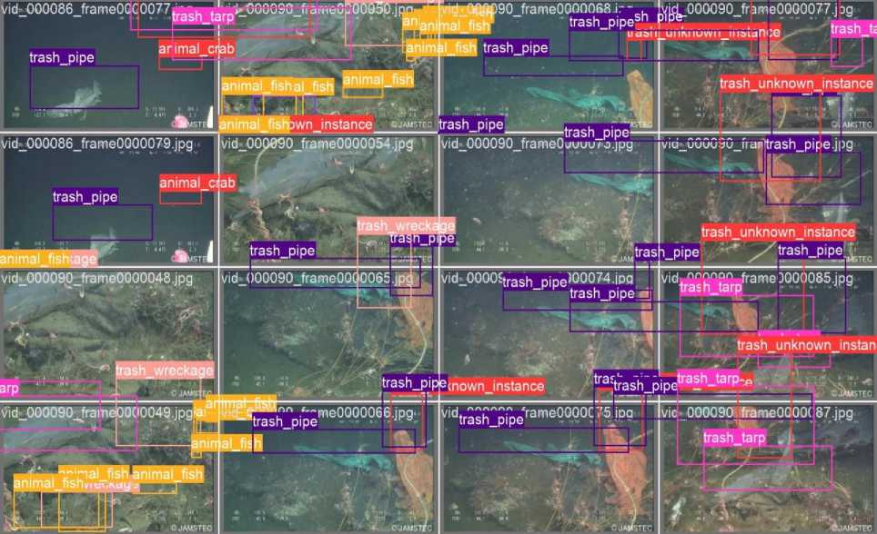
Fig. 3. Instance Version Result with YOLOV8

The architecture of YOLOV8 is significantly faster, and more accurate than previous versions of YOLO. YOLO is a convolution neural network with 24 convolutional layers followed by 2 fully connected layers. YOLOV8 is a single stage object detection model that can be divided into three parts: the backbone, the neck, and the head. Backbone which is also known as the feature extractor, captures simple patterns such as edges and textures and generates a rich, hierarchical representation of the input. YOLOv8 uses modified CSPDarknet53 as the backbone network. This architecture consists of 53 convolutional layers.

The Neck which is a bridge between the backbone and the head, performs feature fusion operations. The Neck basically collects feature maps from different stages of the backbone.

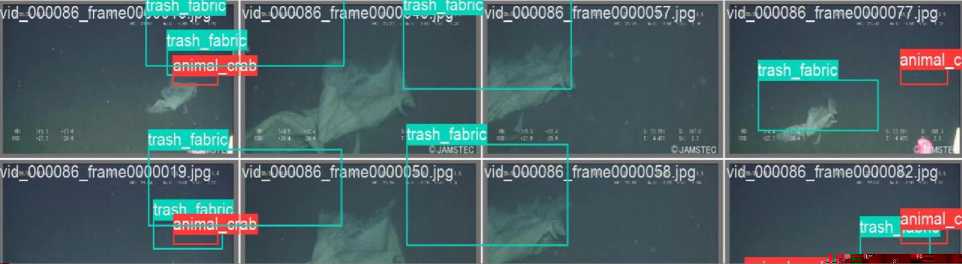
Fig. 4. Material Version Result with YOLOV8

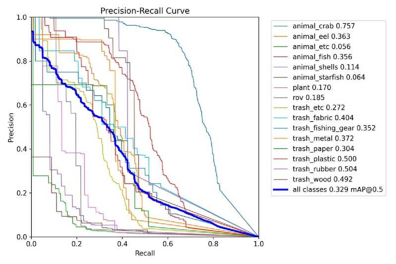
Fig. 5. Precision and Recall with Material Version

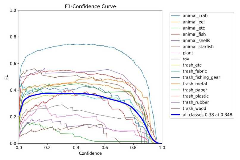
Fig. 6. F1 Confidence Curve with Material Version

The head finally generates the network’s outputs, such as bounding boxes and confidence scores for object detection. The head of YOLOv8 consists of multiple convolutional layers followed by a series of fully connected layers. These layers are responsible for predicting bounding boxes and class probabilities for the objects detected. YOLOV8 introduces anchor free detection head. Previous versions of YOLO were anchor based. These models utilize predefined anchor boxes, which are essentially templates for various shapes and sizes that an object can have. These anchor boxes guide the model in predicting the location of objects within an image. Whereas, an anchor-free model like YOLOV8 does not use these predefined anchor boxes to predict objects. Instead, it predicts bounding boxes directly from the features extracted from the input image. This makes YOLOV8 more flexible in detecting objects of different shapes and sizes, particularly thin or small objects that may not fit well within the predefined anchor boxes of an anchor-based system. An additional benefit of the anchor-free approach is its simplicity. By removing the reliance on anchor boxes, the model becomes easier to understand and implement. YOLOV8 has five versions: yolov8n-nano version, yolov8s-small version, yolov8m medium version, yolov8l- large version, and yolov8x - extra-large version. In this implementation we have used large version of YOLOV8.

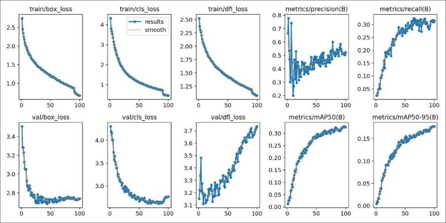
Fig. 7. Results with Material Version

• 3.2.    Baseline Methods

• 3.3.    Dataset

YOLOv8 uses modified CSPDarknet53 as the backbone network, PAN-FPN structure as Neck, and Anchor-free head predicts object centers and box dimensions directly, without predefined anchors. YOLOv8 shows improved performance for small and densely packed objects.

Performance of anchor-free YOLOv8 model is compared with the anchor-based models YOLOv3 and YOLOv5.

YOLOv3 Uses Darknet-53, backbone. For anchor-based detection head in YOLOv3 model, each grid cell predicts bounding boxes relative to predefined anchor boxes. It uses multi-scale prediction and detects at 3 different scales, where, each detection scale results in 9 anchors, with 3 bounding boxes per cell.

YOLOv5 uses CSPDarknet53 (Cross Stage Partial networks) as the backbone, PANet (Path Aggregation Network) as Neck and Anchor-based detection head same as YOLOv3. Anchor-based head predicts bounding boxes relative to anchors. Each scale predicts multiple boxes per grid cell. Similar to YOLOv3, detects objects at 3 scales: small, medium, large.

Anchor-free heads offer a simpler and more efficient alternative, with notable strengths in detecting small and densely packed objects, while anchor-based heads suffer from anchor hyper-parameter dependence, higher computational overhead, and limited adaptability across diverse datasets.

The task of data collection for the task of underwater debris detection is challenging. Data need to be captured under seawater at the maximum depth with high-definition cameras. The lack of sunlight in the deep sea results in uncertainty while collecting debris data samples. The presence of marine life, animals and plants, rocks, algae, and marine flora and fauna makes it difficult to distinguish and identify the marine litter.

Dataset used in this implementation is Trashcan [25]. TrashCan 1.0 is an open-source and well-documented dataset. Original source of the TrashCan is the J-EDI (JAMSTEC E-Library of Deep-sea Images) dataset, generated by the Japan Agency of Marine Earth Science and Technology (JAMSTEC). This is a dataset, containing 7,212 images with different types of trash, plants, and animals. TrashCan 1.0 includes a wide range of debris types — plastic, metal, rope, net, wood, glass, paper, and also non-trash classes like fish and ROVs. There are two versions of this dataset having images and annotations stored in JSON file: the material version in which classes are defined by the material of the trash and the instance version in which classes are defined by the type of object of the trash. As shown in table 4, the instance version is having 22 classes and the dataset is split into training (83%) and validation (17%) sets. The material version is having 16 classes and the dataset is split into raining (84%) and validation (16%) sets. Trashcan dataset is in COCO JSON format. Dataset is in two parts: images and annotations. Images are organized in a hierarchy of directories: main directory containing three sub directories, Train, Validation and Test. Annotations are in JSON format. The JSON file for Material version and Instance version is stored in main directory. The COCO dataset is formatted in JSON. The JSON file is a dictionary of keys: “info”, “licenses”, “images”, “annotations”, “categories” and “segment info”. The annotation format is category id, followed by the bounding box values. The annotation file for each image is generated using the JSON file.

Table 4. Trashcan Dataset

Dataset	No. of Classes	Train	Val
Instance	22	6065	1147
Material	16	6008	1204

Table 5. Models Implemented

OLO Version	YOLO Model	Backbone	Neck	Detection Heads.	Model Variants
YOLOV5	yolov5m	CSP-Darknet53	PANet	detection layer 1 : 80 x 80x 256 for detect small size object detection layer 2 : 40 x 40 x 512 for detect medium size object detection layer 3 : 20 x 20 x 512 for detect large size object.	YOLOv5x, YOLOv5l, YOLOv5m, YOLOv5s, YOLOv5n.
YOLOV3	yolov3u	Darknet-53	FPN	detection layer 1 : 52 x52x 256 for detect small size object detection layer 2 : 26 x 26 x 512 for detect medium size object detection layer 3 : 13 x 13 x 1024 for detect large size object.	YOLOv3, YOLOv3-Ultralytics, YOLOv3u
YOLOV8	YOLOV8l	CSP-Darknet53	FPN+PAN	detection layer 1 : 80 x 80x 256 for detect small size object detection layer 2 : 40 x 40 x 512 for detect medium size object detection layer 3 : 20 x 20 x 512 for detect large size object.	YOLOV8n, YOLOV8s, YOLOV8m, YOLOV8l, YOLOV8x

Table 6. Results of Models Implemented

Model	mAP	Recall	Precision
YOLOV3	0.31879	0.31028	0.78615
YOLOV5	0.43608	0.42033	0.82977
YOLOV8	0.5095	0.49388	0.87811

• 3.4.    Experimental Environment

  12th Gen Intel Core i9-12900K × 24 processor, Operating system: Ubuntu 20.04.6 LTS, GPU: NVIDIA RTX A4000 with 16GB. Ultralytics with Pytorch CUDA version 12.1 (torch-2.1.2+cu121) and Python-3.11.5 is used. Hyperparameters used in the implementation of models is listed in Table 7.

• 3.5.    YOLO Model Implementation and Results

4.    Conclusion

Table 7. Training Hyperparameters for YOLOv8 Model

Hyperparameter	Value / Setting
Image size ( imgsz )	640
Epochs	100
Patience	50
Batch size	16
Device	CUDA
Workers	8
Optimizer	AdamW / SGD with momentum
Verbose	True
Seed	0

Table 5 lists all the details of YOLO models (YOLOV8, YOLOV5, YOLOV3) that are implemented in this work for underwater debris detection task using the TrashCan 1.0 dataset. Table 6 gives precision recall and mAP values for the three models. For implementation of these models Ultralytics is installed and the models are imported from Ultralytics. The performance of three YOLO models, YOLOV8, YOLOV5 and YOLOV3 is evaluated on Trashcan Instance version and Material version dataset. For the training of the YOLO model, number of Epochs used are 200, Patience Parameter is 50, and Batch Size is 16. For the YOLO model validation, best weights recorded during the training of the model are used.

Water bodies across the globe play a crucial role. The micro plastics, formed by dumping plastic, enter the food chain and pose harmful threats to humans and the ecosystem. The widespread issue of underwater debris continues to put these ecosystems at risk. Project aim is to build a Deep Learning Model for Underwater Debris Detection. Major objectives of the work carried out in this research are, implementation of Deep Learning models for Underwater Debris Detection, improvement in performance of Deep Learning Models in identifying marine debris in underwater images and videos, and a comparative analysis using various models available. In this implementation, one stage debris detection and classification using object detection module based on deep CNN is used with the backbone or feature extraction and feature fusion module. Implementation is carried out on TrashCan 1.0 dataset which is divided into : Instance Version and Material Version. Performance of YOLOV3, YOLOV5 and YOLOV8 is compared in this implementation. YOLOV8 outperformed the baseline methods in this implementation.