Application of Adaptive Neural Network Observer in Chaotic Systems

Published Online January 2014 in MECS

Chaos phenomenon is addressed in various fields of engineering and several multi-disciplinary subjects. Chaos may be of a beneficial phenomenon like circuit secure telecommunication [1], although the chaos has a destructive effects in physical and practical applications. Due to complicated dynamic of such these systems, identification and/or the estimation may fail to comply with the needs. Furthermore when there is lack of enough prior information where two approaches are possible:  1) Using a controller to cope with uncertainties of system [2]. 2) Or gaining an observer in the close loop path of the system. Accordingly an adaptive neural network is presented in this study to estimate chaotic states even an online use. This ability helps designer to control chaotic system with satisfactory performance.

Different observers are presented to construct a proper structure to estimate states of systems. This includes nonlinear observers such as EKF and UKF [47].

A first nonlinear adaptive observer was presented in [8] whereas several other observers were proposed in [9-11]. In the current study an adaptive neural network observer will be used when the weights are tuned online [12]. A key issue in using neural networks is the method of training networks. Training process can be performed either online or offline. The proposed observer will be online trained whilst there is no need of prior knowledge about nonlinear terms during the estimation procedure.

This paper is organized as follows:

Neural network will be briefly explained in section two. In section III characteristic of the adaptive observer will be described. The observer will be used to estimate state of a chaotic pendulum system in section four. The work will be continued to observe states a modified Duffing system. Finally a conclusion ends the discussion at section V.

• II.    Brief review of Neural Networks

Neural network is inspired from biological system. Preliminary a schematic form of neural network is shown in Fig. 1.

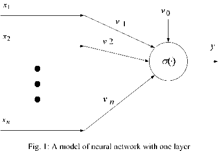
where the input and the relevant weights vectors of neural network are:   x = [x 1 x 2.........xn ] and v = [v 1 v 2.........vn ] respectively. The output is denoted by y whilst v0 is a bias term. The activation function is also shown by ст which may be of a step function, purelin or a sigmoid transfer function.

Output of neural network with one layer is stated by the following equation:

n

y ^{( t} ) = ^{c (} ^ v j x j + v 0 )                      ⁽¹⁾

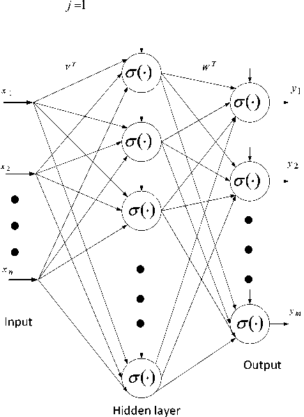
Fig. 2: A two-layer neural network model [12]

In order to model the behavior of complex system, neural network structure will be enhanced. A first kind of promotion will be taken places when the number of layers and neurons of neural network are increased. According to this purpose, the concept of is demonstrated. A structure of multi-layer neural network using two layers is presented in Fig. 2.

Although a two-layer neural network is beneficial, using three layers with sufficient neuron in hidden layers is found effective to simulate most of nonlinear systems.

• III.    Adaptive Neural Network Observer

In this section a structure of adaptive neural network [12] will be described. Consider the following single input-single output nonlinear plants when pair of ( A , C ) is observable:

x = Ax + b [f ( x ) + g ( x )u + d (t )] y = C T x

Where x e R n , y e R , u e R and b e R n are states, output, control signal and its coefficients whereas d ( t ) (is an unknown disturbance with known upper bounded.

Terms f , g : R n ^ R denote unknown smooth nonlinear functions. Apart from, the linear term is also defined in a canonical form which as in the following:

x = Ax y = CT x

Where:

0 1  0 ... 0

0 0  1 ... 0

C =

0  0 ...  1  0

A nonlinear state observer proposed as follows:

x = Axe + b [ f (. x ) + g; ( x ) u - v ( t )] + k [ y - C^T et]

T y = C x

where x ˆ denotes an estimation of state x whereas

T such that the term (A - KC ) must be strictly Hurwitz. Term v (t) provides a robust term of observer to reduce effects of disturbance on system. The rest of variables are the same as in (3). In the following the observer design is presented.

The estimation error is defined by:

x = x - x                                   (6)

This immediately yields the estimation error dynamic which is as follows:

Constant parameters in (10) are tuned to guaranty the observer stabilization to estimate those relevant nonlinear terms.

x = ( A - KC^T ) x + b [f + gu + d (t ) + v (t )] y = C T x

Where ^f = ^{f ( x} ) - ^{f (} x ) and g = g ( x ) - g ( x ) define relevant error terms from that of the original. The design takes place by tuning the observer gain K such that A -KC to become stable. It is the aim to use a neural network to estimate nonlinear terms of the system in an on-line train scheme. The applied neural network [12] observer involves two layers which is described with the following equation:

IV. Application4.1 Chaotic Pendulum System

In this section, the proposed approach will be implemented on a pendulum system. Consider the following state space representation of pendulum system assuming x (0) = [0  0] as an initial condition

[13]:

f ( x ) = W^T ^ V^Tx) + _e

In simulation procedure the first layer is considered as V = I s _x r where s and r denote number of the input and the output layers, respectively. The activation functions in the first and second layer are the sigmoid and the purelin functions respectively. These form the nonlinear equation which is as follows [12]:

x 1 = x 2

x 2 = - sin x 1 - a x 1 - 5 x 2 + f (t ) + d (t )

where f (t) = (a - ^2) a1 cos(^t) - 5coa1 sin (rot)

+ sin ( a 1 cos( ro t ) + a ₀) + a a₀

Where and d ( t )  is disturbance. The

dynamic

f ( x ) = W T O f ( x ) + E f g ( x ) = w g O g ( x ) + E g

Biases of both two functions are considered zero. Meanwhile training of the network needs a series of data in order to tune parameters during the training procedure.

In fact, in [12]; an equation is proposed for training the network to maintain the stability of system. Outcome of this equation provides the weight coefficients of the system at any circumstances. Training of this neural network for two nonlinear terms is achieved from the following differential equation:

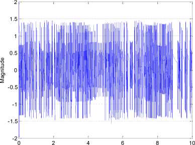
using a = 0.5 , a = 0.3 , 5 = 0.12 , ro = 0.75 , a ₀ = -3 is of chaotic with the phase portrait in Fig. 3.

In order to become more practical, the nonlinear term of the plant is assumed unknown whilst the first state of plant, i.e. x ₁ , is also available. It should be noted that this observer as a full order observer is able to reconstruct all states. However the other available states are used to configure the correction term i.e. v . An aim is to estimate some states using neural network observer in presence of external disturbance. The state x ₁ and the estimation are accordingly shown in Fig. 4.

W f = F f O f y - k f F f |y| W f

^Wg = ^Fg ^O g y ^u - ^kg^Fg l y l ^Wg

^Ff , F g , K f

and K g are constant parameters of

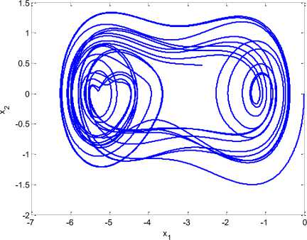
Fig. 3: Chaotic behavior of pendulum system in 250 seconds

equation which must be tuned to determine desired weights. Meanwhile о is a sigmoid activation function as in:

о = o( x) =

1 + exp( - x )

actual

estimated

0.6

actual

0.4I                                                    I ~ ~*~~ estimated

• --00⁰..^.42⁰²

• -^-0⁰.^._-18⁶

• -1.2

  -1.4

0      1      2      3      4      5     6      7      8      9     10

time (sec)

Fig. 4: State trajectories x 1 , x 1

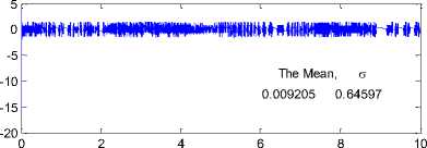
The estimation procedure results the estimation error of x ₁ as shown in Fig. 5.

Time (Sec)

g. 5: Estimation error of x 1

Fi

The procedure will be in progress to estimate the second state continued i.e. x ₂ .

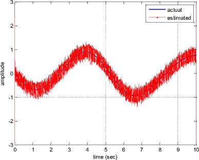
Fig. 6: State trajectories x 2 , x 2

Although the second term in (12) i.e. x2 is more complex, the performance of the observer is found acceptable. This essentially confirms the capability of the proposed observer.

hiiiiii min

-⁰¹1 mu mu

-2

• -3

• -4 t [ 1 [ 1 1

0 2 4 6 8 10

Time (Sec)

• Fig. 7:    Estimation error of x 2

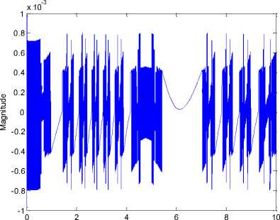
According to the observer performance, the estimation error of second state is shown in Fig. 7. Meanwhile a frequency analysis of the error will be given here for the worst case i.e. x ₂ error in Fig. 8.

The correction term is provided by means of the estimation error. However an appropriate produced error is shown in Fig. 7. First few samples of the estimation seem unrealistic. This is due to choosing different initial condition for the observer from that of the real state. In fact the correction term needs some times i.e. the first few samples, to be settled against discrepancy of the initial conditions from that of the real.

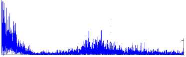
In order to assess the realizability to gain in the closed loop, a spectral frequency analysis is made as shown in Fig. 8.

Power Spectral Density, PSD

The most 3 highest harmonic

The PSD , The Frequency (Hz)

49.2567   0.09999

35.7795   0.19998

20.2038   0.29997

100        200        300        400        500

Frequency (Hz)

• Fig. 8:    Spectral analysis of the complete estimation error

• 4.2 Modified Duffing System

As it can be seen there is almost a big energy (49) in 0.1 Hz, which dominates the rest of response. To find further components the frequency analysis, the frequency analysis is gone further by choosing some other parts of the signal. This results no more success which means intermediate signals are also realizable.

The capability of the proposed observer will be investigated on another second order chaotic Modified Duffing system. Consider the following state space equation of the system, considering x (0) = [2 1] as an initial condition [14]:

x 1 = x ₂

x ’ ₂ = - px 1 - qx ³1 - (a + b cos( ^ t )) x ₂ + d (t )

Where d ( t ) stands for the disturbance. Similarly the system will be of chaotic p = - 1 , q = 1, b =- 1, to = 1, a = -0.001where can be seen is the phase portrait in Fig. 9. The assumption in the last section will be similarly again made. This means that the system state x ₁ , is measurable whilst the nonlinear term of the system is not identifiable.

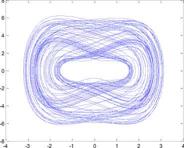
Fig. 9: Chaotic behavior of modified Duffing system in 250 seconds

Figure 10 depicts the states and that of the estimated.

actual estimated

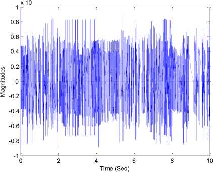
Fig. 11: Estimation error of x 1

The estimation process will be continued to reconstruct the second state, which can be seen in Figure 12. The nonlinearity of the system is mostly occurred on the second state. Therefore the estimation of the second state is challenging. However Fig. 12 shows the estimation result of using the proposed observer.

Furthermore performance of the proposed observer is verifies as the estimation error is seen in Fig. 13.

-1

-2

-3

-4

-5

34567 time (sec)

8      9     10

Fig. 10: State trajectories x 1 , x 1

As seen from Fig. 10, the outcome of the estimation of the states is satisfactory. The estimation error of x ₁ can also be seen Fig. 11.

Time (Sec)

Fig. 13: Estimation error of x 2

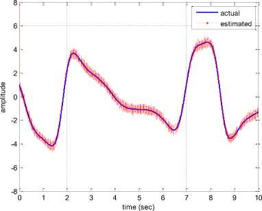
Fig. 12: State trajectories x 2 , x 2

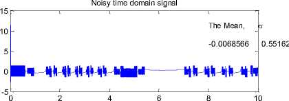
The same frequency analysis is made for the estimation error. Since the estimation error of the second state (Fig. 13) is more challenging, an analysis is done for this error using the fft command in MATLAB^TM software. The frequency spectrum and that of the processed data is shown in Fig. 14. As shown in the figure dominant frequency are located at the lower region i.e. below 10 Hz. Similar to that of in the first case, i.e. the pendulum, most of the energy is condensed at low frequency e.g. 5 Hz. This confirms the proposed observer is realizable. Unlike to the first case there are higher components with almost lower energy. This may be caused by the higher nonlinear term in the model. However this may be filtered by the process itself.

Noisy time domain signal

7.3727

7.3156

7.2792

0.89991

2.5997

5.8994

Power Spectral Density, PSD

Elapsed Time = 0.138 Sec The most 3 highest harmonic The PSD , The Frequency (Hz)

Frequency (Hz)

Fig. 14: Spectral analysis of the most part of the control effort

• V. Conclusion

In this study, an adaptive neural network based observer is proposed to estimate states of a complex chaotic system. The procedure is found capable of being realized in practical systems. Apart from few first samples spectral frequency analysis verifies the proposed observer is realizable. Cure of the shortcoming in some few instances of the frequency is promising by choosing less discrepancy of the initial conditions of the estimation procedure and also filtering characteristics of the process. The neural network tunes the weight of the connection from each node from the first layer to the second. This structure appropriately approximates unknown nonlinearity in the system dynamics. The observer found capable to estimate the chaotic system states.

In this paper, the observer procedure is primarily implemented on a chaotic pendulum system with complex and nonlinear dynamic. The work is continued to estimate states as well as the unknown nonlinear terms of the chaotic modified Duffing system. A frequency analysis is also performed to verify the generated control effort is realizable. Simulation results confirm the performance of the proposed structure of the sensor-less control of chaotic systems.