Application of an enhanced self-adapting differential evolution algorithm to workload prediction in cloud computing

Published Online August 2019 in MECS

Cloud computing is developed to provide on-demand computing services for the customers via the Internet, through web-based tools and applications, rather than having local servers or personal computing resources. The word "Cloud" refers to the servers that are connected to the Internet and represent data centers for computing services [1]. Cloud computing has many advantages like high flexibility, scalability, robustness, and cost saving [2]. It relies on virtualization technologies that offer virtual services, such as hardware virtualization and software virtualization, to share different computing resources among the customers and concurrently execute several work requests. Cloud computing has three main services: Software as a Service (SaaS), Platform as a Service (PaaS), and Infrastructure as a Service (IaaS) [1, 2]. In the SaaS, several software applications are provided to the clients. Every application can be accessed by multiple clients at the same time and each one is isolated from other clients. In the PaaS, the cloud computing provides the clients with a platform to develop applications and services. In the IaaS, physical or more often virtual computing resources are provided as a service to the users. Resource management is an important issue in the IaaS cloud service models that affects the efficiency of the cloud computing [2]. Workload prediction techniques are required to manage the cloud resources and increase the performance of the cloud computing [3]. According to the prediction of the workloads, resources are scaled up or down automatically to balance the workload among the computing resources. The resource scaling efficiency depends on the utilized workload prediction method. The future workload prediction methods are classified to statistical methods[4] and machine-learning methods [3]. In the statistical methods, the prediction is done by matching the current workload history with the similar workload in the past. Therefore, these methods are suitable for short-term workload prediction. They have a poor performance for long-term workload predictions [3]. In the literature, there are several statistical methods that have been applied to the workload prediction in the cloud such as: moving average [5], linear regression [6], Monte Carlo [7], and quadratic regression [6]. In the machinelearning methods, historical information about the previous workload is used to design a predicted model for the future workload. They overcame the problem of dealing with the long-term workload prediction that is suffered by the statistical methods [3]. There are several machine-learning methods that have been applied to the workload prediction in the literature such as: support vector machine (SVM) [8], regression tree [9], and artificial neural network (ANN) [10-12]. In the present paper, we propose a workload prediction approach for cloud computing using artificial neural network and an enhanced self-adapting differential evolution algorithm (MSaDE) [17]. This paper is organized as follows. Section II presents an overview of the related work. The MSaDE algorithm is reviewed in section III. Section IV presents the workload prediction approach. In Section V, the approach is tested through two different benchmark datasets. Finally, Section VI concludes the paper.

• II.    Related Work

Recently, various prediction approaches have been proposed to predict the future work-load per-server required. In [13], an adaptive approach is developed for workload prediction in the cloud computing applications. The workloads are classified into distinct classes and then each class is assigned to one of the prediction models based on the workload features. The authors in [10] introduce a workload prediction model based on self-adaptive differential evolution (SaDE) algorithm and a neural network to predict the future workloads by extracting the training patterns from the historical information. The SaDE algorithm is used as a learning algorithm for the prediction model. A workload prediction model using long short term memory (LSTM) networks is introduced in [11]. The LSTM network is a special form of the recurrent neural network (RNN). In [14], the authors propose a dynamic workload prediction framework for the web applications using an unsupervised learning method. It analyzes the uniform resource identifier (URI) of web requests using the response time and the size of document features. After that, the distribution of the web requests based on historical access logs is computed to be used in the workload prediction for the future time. In [6], a linear regression model is proposed to predict the workload in service clouds. It uses an auto-scaling mechanism that scales the virtual resources based on the predicted workloads. The authors in [15] use statistical models for the resource requirements prediction in the cloud services. This prediction helps in deployment decisions like capacity, scale and scheduling. In [16], the authors use an adaptive model to predict the future workloads for web applications using support vector regression, linear regression and ARIMA. It uses a heuristic approach to select the model parameters.

In this paper, we use the enhanced self-adapting differential evolution algorithm (MSaDE) [17] to optimize the parameters of the ANN prediction model for cloud computing. Historical information about previous workloads is analyzed to extract patterns according to the prediction intervals. These patterns are used to train the ANN model and predict the future workloads. The MSaDE algorithm is applied as a learning algorithm to improve the prediction accuracy and efficiency of the ANN model for the future workload prediction. The proposed approach is evaluated over two benchmark datasets at different look-ahead times. The results show that MSaDE trains the artificial neural network efficiently to predict the future workloads with high accuracy.

• III.    An Enhanced Differential Evolution Algorithm With Multi-Mutation Strategies And Self-Adapting Control Parameters

  Storn and Price introduced the differential evolution (DE) algorithm in 1995 [18]. DE has been successfully applied to various applications such as pattern recognition, cloud computing, and neural networks [19, 20]. MSaDE is an enhanced variant of the DE algorithm with multi-mutation strategies and self-adapting control parameters. It has been introduced in [17] to dynamically balance the rates of exploration and exploitation and improve the performance of the DE algorithm. MSaDE uses three mutation strategies with their related selfadapting control parameters. The first mutation strategy allows searching search space with a high exploration rate, and the second one allows searching search space with a high exploitation rate, the third one balances exploration and exploitation rates. The trial vector is generated in every generation through the evolution process using only one mutation strategy. The automatic switch between    these    mutation    strategies    during

generations is guided using the best and worst individuals at the current generation. This achieves a dynamic balance between the exploration and exploitation rates, which enhances the accuracy and convergence rate of DE. The three utilized mutation strategies are formed using five randomly chosen

GGGG   G individuals ( X , X , X , X , and X ) as well as the best individual ( X G ) at the current generation G. The base vectors of the first and second mutation are X G and X G , respectively. According to the these mutation strategies, the mutant vector VG+1   (i

= 1, 2, . . . , NP ) is defined as [17]:

'X G + F G X HDF= , if CB G >  CW and rand, [ 0,1 ] <  T

V^{G + 1} i

< XG,, + FG X LDFG, if CBG < CWG and rand, [0,1] > T mean(XG, X^,) + FG x mean (HDFG, LDF°), otherwise.

where NP is the population size, LDF ^G is the difference vector with higher objective function value and HDF^G is the difference vector with lower objective function value. T is a predefined threshold, CB^G = f ( X^G ) - f ( X ^ ,)| , CW =| f ( X^G ) — f ( X* )| , f is the objective function, and m e a n ( ) is the arithmetic mean.

hdf G = <

X

X

G r 2

G r 4

- XG3, if f (XG2 - xG ) > f (XG4 - xG )

- X ^ ,           otherwise.

LDF G = <

XG - xG, ff f (XG - XG3) > f (XG - XG) XG - XG ,         otherwfse.

F ^G , F ^G , and F ^G represent the scaling factors of the mutation strategies. They are randomly chosen for every mutant vector from three predefined ranges. As the performance of the DE algorithm is affected by the control parameter values of the scaling factor F and the crossover rate CR , so, for every mutation strategy, the predefined range is defined for both of the scaling factor and the crossover rate as follows [17]. The range of the control parameter values for the first mutation strategy is defined as F 1 = [0.7 0.8 0.9 0.95 1.0] and CR 1 = [0.05 0.1 0.2 0.3 0.4], such that F G e F 1 and CR GG e CR 1 . The range of the control parameter values for the second mutation strategy is defined as F 2 = [0.1 0.2 0.3 0.4 0.5] and CR 2 = [0.8 0.85 0.9 0.95 1.0], such that F G e F₂ and CR G e CR₂ . The i ,2                                    i ,2

range of the control parameter values for the third mutation strategy is defined as F 3 = [0.3 0.4 0.5 0.6 0.7] and CR 3 = [0.4 0.5 0.6 0.7 0.8], such that F G e F₃ and CR G₃ e CR 3 . Over the optimization process, the control parameters of the next generation ( G+1 ) are updated randomly from the predefined ranges if the trial vector overcomes the target vector in the selection phase. Otherwise, the control parameters are not updated. Switching between the mutation strategies of Eq. (1) is done using the absolute differences CB^G and CW ^G with the probability threshold condition T . For further details about MSaDE algorithm, the complete pseudo-code is given in [17].

• IV.    A Workload Prediction Approach For Cloud Computing

A workload prediction approach is proposed using an artificial neural network (ANN) and the enhanced variant of the DE algorithm (MSaDE) [17]. The prediction model has two phases. In the first phase, the ANN model is constructed with a single hidden layer. In the second phase, the network is trained using MSaDE algorithm. The patterns that are used as inputs to train the ANN model are extracted from the analyzed historical information about previous cloud workloads. The training process is done using the MSaDE algorithm as a learning algorithm to increase the prediction accuracy of the ANN model.

• A.    Workload Prediction Algorithm

A artificial neural networks (ANNs) are widely used in prediction problems because of their high accuracy and efficiency compared to other prediction algorithms [21]. In the proposed prediction approach, we use a single hidden layer neural network trained in a supervised learning manner using the MSaDE algorithm. The neural network prediction model consists of three layers: the input layer, the hidden layer, and the output layer. The number of neurons in the input and hidden layers is determined according to the number of inputs to the neural network prediction model. The output layer has only one neuron that represents the predicted server workloads in future time. We use a linear activation function for the neurons of both input and output layers. The neurons of the hidden layer have a sigmoidal activation function (f) defined as [21]:

^{f (} V ) = <

1 + e ^{- V}

, forhiddenlayer

v ,        otherwise .

where v is the sum of the weighted inputs. The training dataset of the ANN prediction model is created as follows. First, the incoming requests from historical information are extracted. Then the workloads are aggregated according to the prediction intervals and the patterns of workloads are created. Finally, these patterns are normalized within the range [0,1] to form the training dataset of the ANN model. Let WL^t represent the workload vector at the prediction interval t , which is defined as:

WL =₍ wl t    wl^ ••• wl ' ₍)            (5)

where the prediction intervals are assumed to be t = 1, 5, 10, 20, 30, and 60 minutes as in [10]. S is the size of WL^t that represents the overall number of workloads at the prediction interval t . The normalized workload vector WLn^t is calculated using Eq. (6):

WLnt

WL - WL mn

WL max

-

WL min

where WLn1 = (wlnt wlnt • • • wlnL) . WL. и and WLmny are 12 St min max the minimum and maximum workloads in the workload dataset, respectively. The training dataset is utilized in the form of input patterns ( It ) for the ANN model and their corresponding outputs ( Ot ) that represent the future workloads, where It and Ot are defined as:

wlnt wlnt •   wlnM  ^ I = wln2t wlnt wlnM+1 (7) v wlns, - M wlnS, - M+1  • wlnS, _1) Ot = (wlnM+1 wlnM+2  " ■ • wln*sl )T (8) where M is the number of normalized workloads in each input pattern that represents the number of inputs of the ANN model. Fig.1 illustrates the sequence of operations for the proposed workload prediction approach.

• B.    Neural Network Training

MSaDE is an improved variant of the DE algorithm. It has been tested over a wide set of well-known benchmark functions with different properties. The results show that MSaDE has achieved better performance in terms of accuracy and convergence rate compared to other DE algorithms [17]. So we propose to use MSaDE as a learning algorithm to train the ANN prediction model. The training process is considered as one of the optimization problems with dimension D, where D is the number of parameters to be optimized in the ANN prediction model. These parameters represent the synaptic weights of the ANN model. The dimension D is determined as:

D = H x( M + 2 ) + 1           (9)

where H is the number of the neurons in the hidden layer and M is the number of inputs of the ANN model.

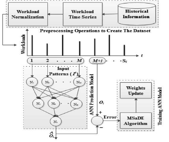
Fig.1. Proposed workload prediction approach

The performance of MSaDE is evaluated by using the mean squared error (MSE) which is the objective function to be minimized,

N

К O i - OO)

MSE = ^--------          (10)

N where N=St - M that represents the number of samples (or input patterns) in the training data set, O is the desired output and ( Oˆ ) is the output of the ANN model.

• C.    Time Complexity of Workload Prediction Approach

The time complexity of the workload prediction approach is based on the time complexity for both the MSaDE algorithm and the ANN prediction model. The time complexity of the DE algorithm depends on the population size (NP), the dimension of the objective function (D), and the number of generations (G). It can be defined as O(G×NP×D). Although MSaDE uses three mutation strategies with their related self-adapting control parameters, its trial vector is generated through generations using only one mutation strategy of these mutations. So MSaDE and DE have the same time complexity. Considering the ANN prediction model, the dimension D is the number of its synaptic weights to be optimized and it is equal to (H×(M+2)+1). Thus, the time complexity for one input pattern becomes O(G×NP×H×(M+2)+1) and it can be approximated to be O(G×NP×H×M). AS H < M, the time complexity can also be approximated to be O(G×NP×M2) as in [10]. Finally, the overall time complexity of the ANN prediction model using the MSaDE algorithm for (N) input patterns is O(G×NP×M2×N). This result shows that MSaDE algorithm achieves the same time complexity as SaDE algorithm for the ANN workload prediction model.

• V.    Experimental Study and Discussion

The proposed prediction approach is evaluated over two benchmark datasets at different look-ahead times, taken from [22]. The dataset 1 represents the workload traces of NASA server and the dataset 2 represents the workload traces of Saskatchewan server. Comparisons are made with two well-known algorithms: the back propagation (BP) algorithm [12] and the self-adaptive differential evolution (SaDE) algorithm [10]. These algorithms are used in [10] as learning algorithms to train the neural network prediction model. The results are assessed in terms of the prediction accuracy represented by the root mean squared error (RMSE) and the average root mean squared error (ARMSE). where RMSE = MSE , and

ARMSE is the average of the RMSE over all prediction intervals. The consumed training time of the ANN model is also investigated. The results of the learning algorithms used for comparison are the same as in [10].

• A.    Experimental Setup

  The experimental results are obtained on a computer with Intel Core i3 processor (2.4 GHz, 3M cache memory) and 4 GB of RAM memory in MATLAB R2007b Runtime Environment. The settings of the ANN prediction model based on the learning algorithms BP and SaDE are the same as in [10], where M =10 and H =7. For the learning algorithm MSaDE, we use two settings for the ANN prediction model. The first setting is the same as in [10] ( M =10 and H =7) and we refer to the MSaDE algorithm as MSaDE1. The population size of the two algorithms MSaDE1 and SaDE have the same population size NP =20. In the second setting, we perform several trials to get suitable values of the parameters M , H , and NP that improve the prediction accuracy of the ANN model. Based on these trials, we found that the appropriate values of M , H , and NP are 5, 3, and 50, respectively. In this setting, we refer to the MSaDE algorithm as MSaDE2. The maximum number of iterations ( G _max) performed by

the learning algorithms BP and SaDE is the same as in [10]. MSaDE1 uses the same value of G _max as SaDE. The different values of G max for the learning algorithms BP, SaDE, MSaDE1 and MSaDE2 over the two training datasets 1 and 2 are listed in Table 1. All experiments are performed over prediction interval values t = 1, 5, 10, 20, 30, and 60 min as in [10]. The first 60% of the dataset is used for training the ANN model and the rest 40% is used for testing it. The results are obtained as the average over 10 independent runs as in [10].

• B.    Accuracy Results

The RMSE values of the results achieved by the learning algorithms BP, SaDE, MSaDE1 and MSaDE2 over the training datasets 1 and 2 are listed in Table 2. The results are plotted in Fig.2 for the two datasets 1 and 2. Comparing MSaDE1 to BP and SaDE, the results show that the prediction accuracy of MSaDE1 is the best through all prediction intervals over the training dataset 1. For the training dataset 2, the accuracy of SaDE is slightly better than MSaDE1 over prediction interval t = 1 and 5 min. MSaDE1 has the best accuracy over the rest prediction intervals t = 10, 20, 30, and 60 min.

Table 1. G max of the learning algorithms over datasets 1 and 2.

Prediction Interval (min)	Dataset 1				Dataset 2
	BP	SaDE	MSaDE1	MSaDE2	BP	SaDE	MSaDE1	MSaDE2
1	250	47	47	250	250	61	61	250
5	250	39	39	250	250	77	77	250
10	250	51	51	250	250	51	51	250
20	250	47	47	250	250	51	51	250
30	250	26	26	250	250	42	42	250
60	250	26	26	250	250	21	21	250

Table 2. Accuracy results in terms of RMSE over datasets 1 and 2.

Prediction Interval (min)	Dataset 1				Dataset 2
	BP	SaDE	MSaDE1	MSaDE2	BP	SaDE	MSaDE1	MSaDE2
1	0.256	0.013	0.011	0.0011	0.119	0.001	0.002	0.0003
5	0.311	0.100	0.039	0.0008	0.336	0.002	0.004	0.0005
10	0.312	0.158	0.043	0.0012	0.313	0.158	0.027	0.0018
20	0.288	0.158	0.047	0.0020	0.329	0.196	0.035	0.0014
30	0.292	0.142	0.057	0.0029	0.349	0.209	0.057	0.0013
60	0.305	0.142	0.063	0.0043	0.323	0.170	0.068	0.0015

Comparing MSaDE2 to BP and SaDE, the results show that the prediction accuracy of MSaDE2 is the best through all prediction intervals over the two datasets 1 and 2. The accuracy results in terms of ARMSE are listed in Table 3, where MSaDE1 and MSaDE2 achieve the best accuracy with a clear difference than BP and SaDE. The consumed training time in seconds of the ANN model based on the learning algorithms over the training datasets 1 and 2 are listed in Table 4. SaDE and MSaDE are population-based optimization algorithms, so they consume larger training time during iterations than the BP algorithm. MSaDE2 consumes less training time than SaDE algorithm over all prediction intervals. The trained

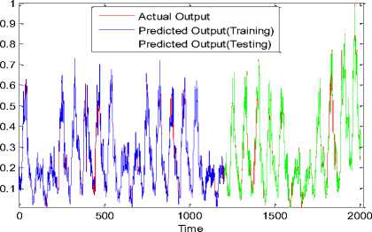
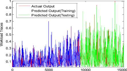
ANN model based on MSaDE2 algorithm will have faster response than other algorithms as it has less number of neurons in the hidden layer and also less number of inputs. Fig.3 shows the predicted workload traces that represent the output of the trained ANN model based on MSaDE2 algorithm and the actual workload traces over the two datasets 1 and 2. The workload traces of this figure are obtained at the prediction interval t = 20 min. It can be observed that the predicted workloads are very close to the actual workloads over the two datasets.

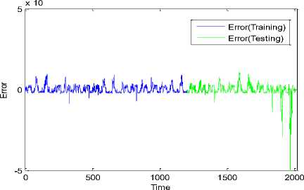
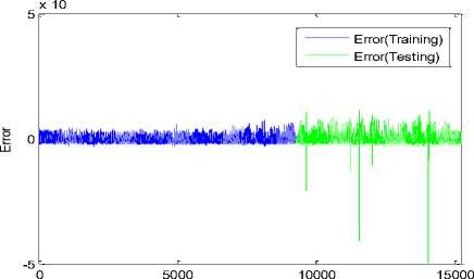
The errors between the predicted and actual output of the ANN model over the two datasets 1 and 2 are plotted in Fig.4.

Workload Traces                                                                                                       RMSE

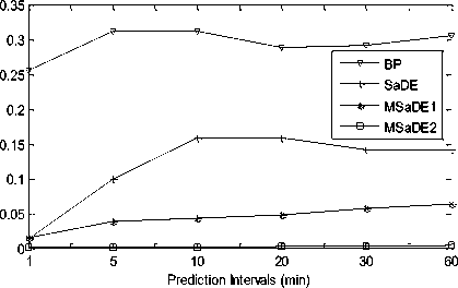
(a) Dataset 1

Fig.2. RMSE vs. prediction intervals over datasets 1 and 2

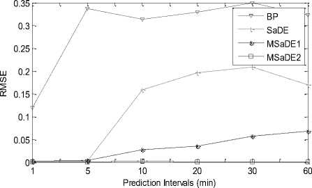
(b) Dataset 2

Table 3. Accuracy results in terms of ARMSE.

Dataset	BP	SaDE	MSaDE1	MSaDE2
1	0.294	0.11883	0.04333	0.00205
2	0.29483	0.12267	0.03217	0.00113

Table 4. Training time in seconds consumed by the learning algorithms over datasets 1 and 2.

Prediction Interval (min)	Dataset 1				Dataset 2
	BP	SaDE	MSaDE1	MSaDE2	BP	SaDE	MSaDE1	MSaDE2
1	121.3	290.8	235.0	175.67	661.6	1949.6	1590.3	1126.6
5	24.11	48.53	41.97	30.45	132.6	498.45	347.26	195.06
10	12.14	31.70	25.32	18.25	64.80	168.66	122.17	96.45
20	6.35	14.75	13.16	10.34	33.37	85.49	62.86	45.31
30	4.27	5.50	7.71	5.22	21.42	46.74	39.34	26.49
60	2.90	3.50	4.31	3.43	10.73	12.23	15.06	11.47

(a) Dataset 1

Time

(b) Dataset 2

Fig.3. ANN model trained by MSaDE2 at prediction interval t = 20 min over datasets 1 and 2

(a) Dataset 1

Time

(b) Dataset 2

Fig.4. Error of ANN model trained by MSaDE2 at prediction interval t = 20 min over datasets 1 and 2

• VI.    Conclusions

In this paper, we propose a workload prediction approach based on an artificial neural network (ANN) and an enhanced variant of the DE algorithm denoted by MSaDE. To show the accuracy and responsiveness of the ANN prediction model that is trained by the MSaDE algorithm, comparisons are made with two different learning algorithms: the back propagation (BP) algorithm and the self-adaptive differential evolution (SaDE) algorithm. Comparisons are made using two benchmark datasets over different prediction interval values ( t = 1, 5, 10, 20, 30, and 60 min). We use two settings for the ANN prediction model that is based on the learning algorithm MSaDE. MSaDE1 and MSaDE2 are used to refer to MSaDE in the first and second settings, respectively. The prediction accuracy results in terms of ARMSE show that learning the ANN model using MSaDE1 or MSaDE2 achieves high accuracy over datasets 1 and 2 compared to BP and SaDE. Based on the ARMSE values over dataset 1, the percentages of accuracy enhancement achieved by MSaDE1 and MSaDE2 compared to BP and SaDE are 85.26%, 63.53%, 99.30% and 98.27%, respectively. For dataset 2, these percentages are 89.08%, 73.77%, 99.61% and 99.07%, respectively. The performance of the proposed MSaDE2 model depends on two elements: the network structure, and the training algorithm. The MSaDE2 model has faster response than other models as it has less number of neurons in the hidden layer and also less number of inputs. The MSaDE algorithm is used to train the proposed ANN prediction model that improved the prediction accuracy and efficiency of the ANN model for the future workload prediction.

• [1]    A. Prasanth, “Cloud computing services: A Survey,” International Journal of Computer Applications , vol. 46, no. 3, pp. 25-29, 2012.

• [2]    A. Shawish, and M. Salama, “Cloud computing: paradigms and technologies,” in Inter-cooperative Collective Intelligence: Techniques and Applications , N. B. Fatos, Xhafa, eds., Springer-Verlag Berlin Heidelberg,1st edn., 2014, ISBN 978-3-642-35016-0, pp.39–67.

• [3]    K. Cetinski, and M. B. Juric, “AME-WPC: Advanced model for efficient workload prediction in the cloud,” J. Netw. Comput. Appl. , vol. 55, no. 55, pp. 191–201, 2015.

• [4]    Y. Chen, A. Ganapathi, R. Griffith, and R. Katz, “Towards understanding cloud performance tradeoffs using statistical workload analysis and replay,” EECS, UC Berkeley , Tech. Rep., pp. 1-12, 2010.

• [5]    D. Ardagna, S. Casolari, M. Colajanni, and B. Panicucci, “Dual time-scale distributed capacity allocation and load redirect algorithms for cloud systems,” J. Parallel Distrib. Comput. , vol, 72, no. 6, pp. 796–808, 2012.

• [6]    J. Yang, C. Liu, Y. Shang, B. Cheng, Z. Mao, C. Liu, et al., “A cost-aware auto-scaling approach using the workload prediction in service clouds,” Information Systems Frontiers , vol. 16, no. 1, pp. 7–18, 2014.

• [7]    T. Vercauteren, P. Aggarwal, X. Wang, and T Li, “Hierarchical forecasting of web server workload using sequential monte carlo training,” IEEE Trans Signal Process , vol. 55, no. 4, pp. 1286–97, 2007.

• [8]    L. Cao, “Support vector machines experts for time series forecasting,” Neurocomputing , vol. 51, pp. 321–339, 2003.

• [9]    Y. Chen, B. Yang, J. Dong, and A. Abraham, “Timeseries forecasting using flexible neural tree model,” Information Sciences , vol. 174, no. 3–4, pp. 219–3, 2005.

• [10]    J. Kumar, and A. K. Singh, “Workload prediction in cloud using artificial neural network and adaptive differential evolution,” Future Generation Computer Systems , vol. 81, pp. 41–52, 2018.

• [11]    J. Kumar, R. Goomerb, and A. K. Singh, “Long short term memory recurrent neural network (LSTM-RNN) based workload forecasting model for cloud datacenters,” in Procedia Computer Science , sciencedirect , vol. 125, pp. 676-682, 2018.

• [12]    J. J. Prevost, K. Nagothu, B. Kelley, and M. Jamshidi, “Prediction of cloud data center networks loads using stochastic and neural models,” in 6th International Conference on System of Systems  Engineering ,

  Albuquerque, NM, USA, pp. 276–28, IEEE, 2011.

• [13]    C. Liu, C. Liu, Y. Shang, S. Chen, B. Cheng, and J. Chen, “An adaptive prediction approach based on workload pattern discrimination in the cloud,” J. Netw. Comput. Appl , vol. 80, pp. 35–44, 2017.

• [14]    W. Iqbal, A. Erradi, and A. Mahmood, “Dynamic workload patterns prediction for proactive auto-scaling of web applications,” Journal of Network and Computer Applications , vol. 124, pp. 94-107, 2018.

• [15]    A. Ganapathi, C. Yanpei, A. Fox, R. Katz, and D. Patterson, “Statistics-driven workload modeling for the cloud,” in IEEE 26th International Conference on Data Engineering Workshops(ICDEW) , Long Beach, CA, USA, pp.87–92, IEEE, 2010.

• [16]    P Singh., P. Gupta, and K. Jyoti, “TASM: technocrat ARIMA and SVR model for workload prediction of web applications in cloud,” Cluster Computing, Spriger , vol. 22, no. 2, pp. 619-633, 2018.

• [17]    M. A. Attia, M. Arafa, E. A. Sallam, and M. M. Fahmy, “An enhanced differential evolution algorithm with multimutation strategies and self-adapting control parameters,” International Journal of Intelligent Systems and Applications(IJISA) , vol. 11, no. 4, pp. 26-38, 2019.

• [18]    R. Storn, and K. V. Price, “Differential evolution - a simple and efficient adaptive scheme for global optimization over continuous spaces,” International Computer Science Institute(ICSI) , Berkeley, CA, Technical Report, pp. 1-15, TR-95-012, 1995.

• [19]    M. Ramadas, A. Abraham, and S. Kumar, “Fsde-forced strategy differential evolution used for data clustering,” Journal of King Saud University –Computer and Information Sciences , vol. 31, pp. 52–61, 2019.

• [20]    F. Arcea, E. Zamorab, H. Sossaa, and R Barróna, “Differential evolution training algorithm for dendrite morphological neural networks,” Applied Soft Computing , vol. 68, pp. 303-313, 2018.

• [21]    O. I. Abiodun, A. Jantana, A. E. Omolarac, K. V. Dadad, N. A. Mohamede, and H. Arshad, “State-of-the-art in artificial neural network applications: A survey,” Heliyon, Elsevier Ltd , vol. 4, no. 11, e00938, 2018.

• [22]    The datasets NASA and Saskatchewan web server logs are available in http://ita.ee.lbl.gov/html/traces.html .