Application of memory effect in an inventory model with price dependent demand rate during shortage

Author: Rituparna Pakhira, Uttam Ghosh, Susmita Sarkar
Journal: International Journal of Education and Management Engineering @ijeme
Article in issue: 3 vol.9, 2019.
Free access
The purpose of this paper is to establish the memory effect in an inventory model. In this model, price dependent demand is considered during the shortage period. Primal geometric programming is introduced to solve the minimized total average cost and optimal ordering interval. And finally we have taken a numerical example to justify the memory effect of this type inventory system. From the result it is clear that the model is suitable for short memory affected business i.e. newly started business.
Fractional order derivative, Classical inventory model, Fractional order inventory model with memory kernel
Short address: https://sciup.org/15015806
IDR: 15015806 | DOI: 10.5815/ijeme.2019.03.05
Text of the scientific article Application of memory effect in an inventory model with price dependent demand rate during shortage
In last few years, fractional order derivative and fractional order integration has been used to model in different subject of mathematics [1,2,3], economics [4,5,6] to take into account memory effect. It is generally known that the integer order derivatives and integration have clear physical and geometrical interpretation which significantly understands that why they are used for solving applied problems in various topics of science [1,2,3,4,5,6,7,8]. It is known that the time rate of change of integer orders are determined by the property of differentiable functions of time only in infinitely small neighborhood of the considered point of time. Hence, there is assumed an instantaneous change of the marginal output, when the input level changes. Therefore, dynamical memory effect is not present in classical calculus. But in case of fractional derivative the rate of change is affected by all points of the considered interval, so it is a memory dependent derivative [2] .It can illustrate all state of the system. On the other hand, in fractional calculus, the acceptable physical
* Corresponding author:
interpretation of fractional order derivative and fractional order integration is an index of memory. Here we use Caputo fractional order derivative to derive the fractional order inventory model. R-L fractional order integration[9,10] is used to develop the different associated cost. Two types memory indexes have been developed (i) differential memory index, (ii) integral memory index.
Authors expect that inventory model is appropriate to incorporate the memory effect because total inventory system depends on its past experience or past history effect. Most of the time profit of business falls down due to its past history effect like effect of the previous product quality to the customer, attitude of the shopkeeper on the customer etc. Good attitude of the shopkeeper can impress to any customer. Then, its selling rate can increase. Hence, from overall concept we can say that past experience has great impact on the inventory system.
Evaluation of an inventory system with constant demand rate was first considered by F.W.Harris [11].He developed the well-known square root formulae for the economic order quantity of the item. After the pioneering attempt by Harris, several researchers [12,13,14,15,16] have extended different type inventory model. They only developed classical or integer order inventory model. Their focus was not pulled in the direction of fractional order or memory dependent inventory model.
Our purpose is also to develop a memory dependent inventory model with price dependent demand during the shortage period. Numerical analysis has been taken to illustrate the whole fractional order inventory system.
The rest part of the paper has been furnished as follows, In the section-II, the review of fractional calculus has been discussed, Classical inventory model has been given in the section-III, Memory dependent inventory model with analytic calculation has been proposed in the section-IV, Numerical examples have been conducted in the section-V, Graphical presentation has been arranged in the section-VI, at last some conclusions are given to show the effect of the work in the section-VII.
-
2. Related Work
-
2.1. Riemann Liouville Fractional Derivative
There exists vast definition of different definition of fractional order derivative. Some of them, most popular definitions are Riemann-Liouville (R-L) fractional order derivative and Caputo fractional order derivative, Modified left Riemann-Liouville (R-L) derivative.
Riemann-Liouville (R-L) definition[9],[10] of fractional derivative of a th order (where n < a < n + 1 ) for any integrable function f ( x ) on[ a , b ]is denoted RL Dx a ( f ( x ) ) and defined as
D ( f ( x ) ) =
Г ( n + 1 - a )
/ , X n +1 x
( -z i i ( x - o )( n -a ) f (o d ^ к dx ) a
The above results show a difference between ordinary derivative and fractional order derivative. To eliminate this difference M.Caputo [9,10] developed a new definition of fractional order derivative for any differentiable functions.
-
2.2. Caputo Fractional order Derivative
2.3. Fractional Laplace Transform Method
For any differentiable function f ( x ) on [ a , b ] Caputo fractional order derivative [9,10] of a th order is denoted ^ D ^ ( f ( x ) ) and defined as
x cd: (f (x»=-—- /(x - . । n—1—a) f(n) (o d^ I (n - a) a
where ( n — 1 < a < n ).
The Caputo definition has both merit and demerit. Demerit of this definition is that the function should be ( n ) times differentiable otherwise this definition will not valid. On the other hand, themerit of this definition is, Caputo fractional order derivative of any constant function becomes zero where R-Ldefinition fails.
Laplace transformation plays an important role in integer and fractional order differential equations. The Laplace transform of the function f ( t ) [9,10] is denoted by F ( s ) and defined in the following form
to
F ( s ) = L ( f ( t )) = J e — stf ( t ) dt
where s>0 and s is called the transform parameter. The Laplace transformation of integer order derivative is defined as
n — 1
k = 0
where, f n ( t ) denotes
nth order ordinary derivative of f with respect to t .
and for non - integer order a , it is in generalized form as,
n — 1
k = 0
where, a is defined as ( n — 1) < a < n .
2.4. Mittag-Leffler function
G.M.Mittag-Leffler gave a new introduction for generalization form of exponential function in 1903 [23]. This generalization form of exponential function is known as Mittag-Leffler function which plays very spontaneous role in fractional calculus. One parameter Mittag-Leffler function is defined by series expansion
T k
Ea ( ^ ) = £ ^77—7 k=0 r(1 + ak)
It comes from fractional Maclaurin series expansion of the exponential function which is
demonstrated below.
For any continuous fractional derivable function f ( z )has fractional Maclaurin series expansion as
= ^ f (ak)(0) if f (z) is taken as ez. Then it becomes as^ ^z) = ^ zk Two parameter Mittag- k:0r(1+ak) “^ ;“k:0Г(1+ak).
го kk
Leffler function is defined as z a , в ( ) - r ( ek + a )
where a , в > 0
The Mittag-Leffler function has the following properties.
го k
E^- ^ rd+i )
го k
= e , e 2( - ) = У —----
1,2 ( ) :r ( k + 2)
(e z -1) " z k f e- -I- -)
, E 1,3 ( - ) = E ^7 - 7^ 11
- k =0 r ( k + 3 ) -
and generally it can be written as
го к If m - 2 к )
z 1 z z
1, m () k E o r ( k + m ) - m - 1 ( k : 0 r ( k +1 ) J
-
3. Classical Inventory Model
-
3.1. Assumptions
-
The classical model is developed depending on the assumptions
The inventory consists of only one type of items.
The lead time is zero or negligible.
Demand rate is
( a + bt ) for aP - b for
0 < t < t tY < t < T
-
(4) The planning horizon is infinite. (5) Shortage started time is assumed to be fixed.
-
(5) During the stock out period or shortage time, there is complete backlogging.
-
3.2. Notations
-
3.3. Classical Model Formulations
The classical and fractional order inventory model is developed on the base of the notations.
Table 1. Symbols and Items which are used in the Inventory Model.
|
Symbols |
Items |
Symbols |
Items |
|
( i ) I ( t ) |
Inventory level at time t . |
( ii ) C 1 |
Holding cost per unit per unit time. |
|
( iii ) C |
Shortage cost per unit per unit time. |
( iv ) T |
Length of the ordering cycle. |
|
( V )TC a , в |
Total average cost per unit per unit time with fractional effect. |
( vi ) C 3 |
Ordering cost per unit per order. |
|
( vii ) T * |
Optimal ordering interval. |
( viii ) TC * |
Minimized total average cost. |
|
( ix ) h |
Per unit cost. |
( x ) ( r ,. ) |
Gamma function |
|
( xi ) HC ae |
Inventory holding cost with memory effect. |
( xii ) ( B ,. ) |
Beta function. |
|
( xiii ) PC ae |
Purchasing cost per unit time with memory effect. |
( xiv ) SC a , e |
Shortage cost per unit with memory effect. |
|
( xv Кв |
Optimal ordering interval with memory effect. |
( xvi ЖК |
Minimized total average cost with memory effect. |
As the Inventory level reduces due to linear type demand rate during the time interval [0, ^ ] and price dependent demand rate during the time interval [t,T].The classical or memory less inventory system has been governed by the two ordinary differential equations as in the following form d (11 (t)) dt
- ( a + bt ) for 0 < t < tx
(t)
-A2M1 = - ( ap-b ) for t < t < t dt 1
with I ( t ) = 0
We do not want to extend the derivation of the whole classical inventory model because our focus is to develop the memory dependent inventory model or fractional order inventory model.
4. Fractional order Inventory Model with Memory Kernel
To establish the influence of memory effects, first the differential equation (6-7) can be written using the kernels function as follows [1].
^( t ) = -J k ( t - t ') ( a + bt ') dt' dt 0
d^t ) = Дк ( t - 1 ') aP - bdt'
Г ( а - 1)
Using the definition of fractional derivative [9,10] we can re-write the Equation (8, 9) to the form of fractional differential equations with the Caputo-type derivative in the following form
dI ( t ) = - D - ( a - 1) ( a + bt) dt 0 t
dI^t ) =-0 D-< a - 1 )( aP -b )
Now, applying fractional Caputo derivative of order ( a -1 ) on both sides of the Eq. (10, 11) and using the fact the Caputo fractional order derivative and fractional order integral are inverse operators, the following fractional differential equations can be obtained for the model
Here, the strength of memory depends on a . when a ^ 1, memory of the system becomes weak and the small value of a (close to 0.1) indicates long memory of the system.
4.1. Fractional order Inventory Model Analysis
The total fractional order inventory model is governed by the two fractional order differential equation in the following form as
da (I (t))
——- = -(a + bt) for 0 < t < t, da I1 (t))
'./ = -(aP-b) fort, < t < T with I (t,) = 0
Solution of the fractional differential equation is as
I (t ) =
a
Г ( 1 + a )
( t “ - t a ) +
b
( t “ + 1
-
ta+1)
I (t )=
aP - b Г ( 1 + a )
( t ° - t a )
Maximum inventory level is
M = I ( 0 ) =
Г ( 1 + a )( t 1 ) + r ( 2 + a )( t 1 )
Maximum backorder units are
5 = - 1 ( T ) =
aP - b Г ( 1 + a )
( - t a
+ Ta)
Total order quantity is as
Л / х h < лР ° / х
Q - M + S = a ( t^ ) + ° ( +1 ) + aP ( -+ Ta )
Г ( 1 + a )v 4 Г ( 2 + a )v 1 ’ Г ( 1 + a )v 1 ’
Total inventory holding cost is t1
hc ., - C 10 D —в ( I ( t ) )-^ J
I в — 1 I a a a V ° (a + 1
' [цЙ . ( t — ' ' Г 2• a l ( t
—
t a + 1 ) I dt
aCxC x + в
Г ( 1 + a ) Г ( в )
MT'
r ( 2 + a ) Г ( в )
( в is considered as an integral memory index)
Shortage cost is denoted bySC and developed as follows sCa,,-— C, tD- (I (t))-—^ J( T—•)'"[р^ (ta—ta)]dl
_ C , aP - ° |I _1 ( , — 1 ) ) , , (( в - 1 ) t " *2 ) —2 _ j t^ , —1 _ ( t o) , , a + 2 r , —1
Г ( в ) Г ( 1 + a ) (( ( a + 1) ( a + 2 ) J ( a + 2 ) ( a + 1 ) ( в ) ( )
Therefore, total purchasing cost is as
P = h - Q = h L•(l a 1 . , ( t )
____° ____G a +1)
Г ( 2 + a ) ( 1 )
+
aP - ° Г ( 1 + a )
( — t ° + T a )
( Q is substituted from the equation (20)) Therefore, total average cost is as
_ ( PCa , в + H C a , в + S C a , в + C 3 ) TC a , в =
T
I I nt“ ht“ лР^°a ) ) ИлР ° h ,at1 x + —Tt— — t\ + C + HCa6 T + TTa
( (г ( 1 + a ) Г ( 2 + a ) Г ( 1 + a ) J 3 a ' в J Г ( 1 + a )
+ C 2 aP ° Г ( в — 1 ) ), + в —1 + C 2 ap ° ( ( в — 1 ) t a +2 ) т р —3
Г ( в ) Г ( 1 + a ) ( ( a +1 ) ( a + 2 ) J Г ( в ) Г ( 1 + a )( a + 2 )
Г CaP~ ° a +1
чГ ( в ) Г ( 1 + a )
C . aP ° ( t a +l ) L в —2 _ C 2 aP- ° t 1 -
Г ( в ) Г ( 1 + a )( 1 + a ) J Г ( в + 1 ) Г ( 1 + a )
( HC , PC , SC are substituted from the equation (21),(22),(23) respectively)
Case-1: 0 < a < 1.0,0 < в < 1.0.
In this case, the inventory model can be written as follows
A= C 2 aP" f ( в -1 ) ) B . C 2 aP" b ((в — 1 ) t + 2 )
c = f C 2 aP- b t a +1 _ C 2 aP~ b ( t “ + 1 ) ) D = _ C 2 aP- b t “
-
(a) Primal Geometric Programming Method
To solve (25) analytically, the primal geometric programming method has been applied. The dual form of (25) has been introduced by the dual variable ( w ).The corresponding primal geometric programming problem has been constructed in the following form as,
f A ) w1
f B ) w2
I w1 V
I w2 )
w 3
C
l w3 J
w 4 w 5
D - l w4 J l w5 J
w 6
- l w6 J
Normalized condition is as
Orthogonal condition is as
(a + в -1) W +(в - 3) w2 +(в - 2) w3 +(в -1) w4 +(a -1) w5 - w6 = 0 (28)
and the primal-dual relations are as follows
AT a + в - 1 = wd ( w ) , BT в - 3 = wd ( w ) , CT в - 2 = wd ( w )' DT в - 1 = wd ( w ) , ET" - 1 = w5d ( w ) , FT - 1 = wd ( w )
Using the above primal-dual relation the followings are given by
B1w1 Aw
( „ Л a +2 л
B1 w3 Cw4 _ B1 w3 Ew4
I Cw2 I , Dw I Cw2 I, Dw
2 3 25
в -°
Bw Fw
A a
B
I Cw2 J
along with
B1w3 Cw
Solving (27), (28) and (30) the critical value w *, w *, w *, w *, w *, w * of the dual variables w , w , w , w , w , w can be obtained and finally the optimum value T* of T has been calculated from the equation of (31) substituting the critical values. Now the minimized total average cost TC * has been calculated by substituting T * in (25) analytically. The minimized total average cost and the optimal ordering interval is evaluated from (25) numerically.
Case-2: 0 < a < 1.0, в — 1.0.
In this case, the inventory model can be written as follows
'Min TC , ( T ) = AT a + BT 2 + CT - 1 + DT 0 + ET a - 1
Subject to T > 0
C 2 aP — b I 1 B — 0
Г ( в ) Г ( 1 + a ) ( ( a +1 ) J 1
C —
C2aP - b t ? + 1
Г ( 1 ) Г ( 1 + a )
C2aP — b t“ +1) ) Г Г Qf bta aP-bC )
1 + h at 1 + bt 1 — aP t 1 c + hc
Г ( 1 ) Г ( 1 + a )( 1 + a ) |r ( 1 + a ) Г ( 2 + a ) Г ( 1 + a ) J 3
C 2 aP - bt a haP - b
.E T
Г ( 2 ) Г ( 1 + a ) Г ( 1 + a )
In similar way using primal-geometric programming method as case-1, the minimized total average cost and the optimal ordering interval can be obtained from (32) analytically.
Case-3: 0 < в < 1.0, a — 1.0.
In this case, the inventory model can be written as follows
'Min TCX p ( T ) — AT в + BT в - 3 + CT в - 2 + DT в - 1 + ET 0 + FT - 1
Subject to T > 0
' C^aP" b t 2 _ C 2 aP~ b ( t 1 ) 1 __ CaP~ b t,
Г( в )Г( 2) Г( в )Г(2)( 2)J, = Г( в + 1)Г( 2)
haP _
Ж,
h
at, bt, aP b tx
+ C + HCtJi
In similar way as case-1, the minimized total average cost and the optimal ordering interval can be obtained from (33) analytically.
In this case, the inventory model can be written as follows
A = C\P ( A f11, B* = 0, Г(1)Г( 2)( 2 J 1
C =
CaP - bt 22 C 2 aP - b ( t 2 )
Г(1)Г(2) Г(1)Г(2)(2)
, | at bt aP bt}
+ h1
( (r(2) Г(3) Г(2)
+ C + HC
CaP - bt haP - b
E = γ ( 2 ) Γ ( 2 ) γ ( 2 )
In similar approach as case-1, the minimized total average cost and the optimal ordering interval can be obtained from (34) analytically.
-
5. Numerical Example
A numerical example has been taken for the fractional order inventory model in proper units.
It is clear from table 2 that for gradually increasing memory effect, minimized total average cost is gradually decreasing. In long memory effect, the minimized total average cost is low compared to the short memory effect. Initially, good business policy is chosen but gradually falls dawn but very slowly.
Table 2. Minimized Total Average Cost and the Optimal Ordering Interval for β = 1.0, and α varies from 0.1 to 1.0 as Defined in Section IV(i).
|
α |
β |
* α , β |
* TC α , β |
|
0.1 |
1.0 |
1.8486x10⁵ |
0.0280 |
|
0.2 |
1.0 |
3.7880x10⁴ |
0.0874 |
|
0.3 |
1.0 |
1.2381x10⁴ |
0.1948 |
|
0.4 |
1.0 |
5.1763x10³ |
0.3652 |
|
0.5 |
1.0 |
2.5442x10³ |
0.6107 |
|
0.6 |
1.0 |
1.4051x10³ |
0.9391 |
|
0.7 |
1.0 |
847.6130 |
1.3550 |
|
0.8 |
1.0 |
547.6867 |
1.8605 |
|
0.9↑(increasing memory effect) |
1.0 |
373.7442 |
2.4570 |
|
1.0 |
1.0 |
266.5016 |
3.1452 |
Table 3. Minimized Total Average Cost and the Optimal Ordering Interval for α = 1.0, and β varies from 0.1 to 1.0 as Defined in Section IV(i).
|
α |
β |
* α , β |
* TC α , β |
|
1.0 |
0.1 |
1.0542x10⁶ |
0.2741 |
|
1.0 |
0.2 |
1.0521x10⁵ |
0.2919 |
|
1.0 |
0.3 |
2.3561x10⁴ |
0.3406 |
|
1.0 |
0.4 |
7.8045x10³ |
0.4421 |
|
1.0 |
0.5 |
3.2981x10³ |
0.6197 |
|
1.0 |
0.6 |
1.6397x10³ |
0.8939 |
|
1.0 |
0.7 |
922.5066 |
1.2797 |
|
1.0 |
0.8 |
569.5749 |
1.7846 |
|
1.0 |
0.9↑(increasing memory effect) |
378.3236 |
2.4087↑( decreasingabove ) |
|
1.0 |
1.0 |
266.5016 |
3.1452 |
It is clear from table3 that corresponding integral memory index, minimized total average cost is gradually increasing with gradually increasing memory effect.
But, from table 2 and 3 it is clear that the optimal ordering interval on or before α = 0.7, β = 0.7 , is much high. Business stay long time to reach the minimum value of the total average cost. This type model is suitable for short memory affected system i.e newly started business.
-
6. Graphical Presentations of Minimized Total Average Cost with Respect to Differential Memory Index and Integral Memory Index.
-
7. Conclusions
Here, Scatter diagrams have been drawn for the minimized total average cost with respect to differential memory index and integral memory index corresponding table 2 and table 3 to show the changing behaviour of the minimized total average cost.
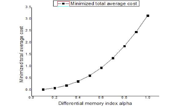
Fig.1. Scatter Diagram for Minimized Total Average Cost with Respect Differential Memory Index α .
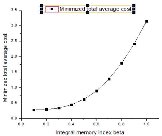
Fig.2. Scatter Diagram for Minimized Total Average Cost with Respect Integral Memory Index β .
This paper presents a memory dependent model with price dependent demand during shortage period. We have considered a numerical example to illustrate the whole model. The numerical example (table 2 and table 3) show that on or before the memory indexes a = 0.7, в =0.7 , business stay very long time to reach the minimum value of the total average cost. It has no real significant in the real market. Hence, we have found that the model is suitable for newly started business i.e short experienced business. Proposed model can further be enriched by taking time delay in payment or more realistic assumptions like probabilistic demand rate.
Acknowledgements
The authors would like to thank the reviewers and the editor for the valuable comments and suggestions. The work is also supported by Prof R.N.Mukerjee, Retired professor of Burdwan University. The authors also would like to thank the Department of Science and Technology, Government of India, New Delhi, for the financial assistance under AORC, Inspire fellowship Scheme towards this research work.
References Application of memory effect in an inventory model with price dependent demand rate during shortage
- Saeedian.M.,Khalighi.M., Azimi-Tafreshi.N., Jafari.G.R.,Ausloos.M(2017),Memory effects on epidemic evolution: The susceptible-infected-recovered epidemic model, Physical Review E95,022409.
- Pakhira.R., Ghosh.U.,Sarkar.S.,(2018) Study of Memory Effects in an Inventory Model Using Fractional Calculus, Applied Mathematical Sciences, Vol. 12, no. 17, 797 - 824.
- Pakhira.R., Ghosh.U., Sarkar.S., “Application of Memory effects In an Inventory Model with Linear Demand and No shortage”, International Journal of Research in Advent Technology, Vol.6, No.8, 2018.
- Tarasova. V.V., Tarasov V.E.,(2016) “Memory effects in hereditary Keynesian model” Problems of Modern Science and Education. No. 38 (80). P. 38–44. DOI: 10.20861/2304-2338-2016-80-001 [in Russian].
- Tarasov.V.E, Tarasova. V.V.,(2016) "Long and short memory in economics: fractional-order difference and differentiation" IRA-International Journal of Management and Social Sciences. Vol. 5.No. 2. P. 327-334. DOI: 10.21013/jmss.v5.n2.p10.
- Tarasov.V.E., Tarasova V.V.,(2017). “Economic interpretation of fractional derivatives”. Progress in Fractional Differential and Applications.3.No.1, 1-6.
- Tarasov.V.E, Tarasova.V.V, Elasticity for economic processes with memory: fractional differential calculus approach, Fractional Differential Calculus, Vol-6, No-2(2016), 219-232.
- Das.T, Ghosh.U, Sarkar.S and Das.S., (2018)” Time independent fractional Schrodinger equation for generalized Mie-type potential in higher dimension framed with Jumarie type fractional derivative”. Journal of Mathematical Physics, 59, 022111; doi: 10.1063/1.4999262.
- Miller.K.S, Ross.B., “An Introduction to the Fractional Calculus and Fractional Differential Equations”. John Wiley &Sons, New York, NY, USA, (1993).
- Podubly.I(1999), “Fractional Differential Equations, Mathematics in Science and Engineering”, Academic Press, San Diego, Calif,USA.198.
- Harris.F.W, Operations and Cost, A. W. Shaw Company, Chicago, 1915, pp. 48-54, (1915).
- Wilson.R.H, A Scientific Routine for Stock Control,” Harvard Business Review, Vol. 13, No. 1; pp. 116-128, (1934).
- Silver.E.A, “A Simple inventory replenishment decision rule for a linear trend in demand”. Journal of the Operational Research Society.30:71-75.
- Deb.M and Chaudhuri.K (1987), “A note on the heuristic for replenishment of trended inventories considering shortages”, J. of the Oper. Research Soc; 38; 459-463.
- Ritchie.E(1984), “The optimal EOQ for linear increasing demand- a Simple optimal Solution”. Journal of the Operational Research Society, 35:949-952.
- Rajeswari.N, Vanjikkodi.T, “An Inventory model for Items with Two Parameter Weibull Distribution Deterioration and Backlogging”, American Journal of Operations Research, 2012, 2, 247-252.
- Ghosh.U, Sengupta.S, Sarkar.S and Das.S(2015). “Characterization of non-differentiable points of a function by Fractional derivative of Jumarie type”. European Journal of Academic Essays 2(2): 70-86.
- Ghosh.U, Sengupta.S, Sarkar.S, Das.S(2015), “Analytic Solution of linear fractional differential equation with Jumarie derivative in term of Mittag-Leffler function”. American Journal of Mathematical Analysis, 3(2).2015.32-38.
- Das.S(2008), “Functional Fractional Calculus for system Identification and Controls”, ISBN 978-3-540-72702-6 Springer Berlin Heidelberg New York.
- Ojha.A.K, Biswal.K.K(2010), “Posynomial Geometric Programming Problems with Multiple parameters”, Journal of computing.Volume-2, Issue-1, ISSN 2151-9617.
- Pakhira.R.,Ghosh.U.,Sarkar.S.,(2018).Study of Memory Effect in an Inventory Model with Linear Demand and Salvage Value, International Journal of Applied Engineering Research, ISSN 0973-4562 Volume 13, Number 20 (2018) pp. 14741-14751.
