Application of Optimized Neural Network Models for Prediction of Nuclear Magnetic Resonance Parameters in Carbonate Reservoir Rocks

Published Online May 2015 in MECS

Porosity, permeability, producible fluid of the reservoir, and irreducible fluid saturation are major petrophysical parameters for reservoir characterization and evaluation. These parameters are derived by different methodologies, including laboratory measurements; well logging, well testing, and core plug analyses. Each of these methods has its advantage and disadvantage and considering several factors and limitations, economical to operational, led to selection of the optimum methodology for obtaining these parameters in a reservoir. Among aforementioned methodologies, well logging is the most popular since its disadvantage are ignorable compared to its advantages. Year by year, new sets of well logging are introduced and make it possible to wider parameters of the reservoir. Nuclear magnetic resonance (NMR) log is one of the potent tools that made a revolution in measurement of reservoir properties that had been impossible to measure before by logging instrument. Permeability, free and bulk fluid of rock that previously measured through time consuming laboratory measurements can be identified by NMR log without the necessity of expensive operation of coring. However, conventional log sets, such as neutron, sonic, resistivity, and density logs, which have been run in all drilled wells, running a NMR log in all drilled wells of a field is a costly task and usually impossible due to economical limitations. NMR log is only run in limited number of drilled wells of field, which has more than dozen of wells. Also, it is impossible to run NMR log in wells that drilled some years ago and already have been cased. The present paper aims to employ the capabilities of supervised intelligent systems for solving these limitations and problems using conventional well logs. Since conventional well logs have been run in all wells of each field, developing a quantitative formulation between conventional well log data and outputs of NMR log can be a reasonable methodology to have a view from the responses of NMR in each well. Studying the previous literatures shows that intelligent models have been diversely used in prediction of reservoir properties [1-6].

Most of previous researches were used neural network, fuzzy logic, and genetic algorithm for developing an intelligent model and obtained acceptable results from designed models. The goal of the present research is not only introduction of an intelligent model for prediction of NMR log’s outputs but also it tries to benefit from the advantage of three optimization models, including genetic algorithm (GA), particle swarm optimization (PSO), and ant colony optimization (ACO) in designing the neural network model. The performance of three optimized network is studied in terms of prediction error and convergence time of optimization model. The paper is organized as follow. The next section introduces the significance of NMR log and its outputs in detail. This section clarifies the importance of NMR log in reservoir characterization. The principals of neural network models and employed optimization algorithms are discussed in the third section. The next is application of developed models in a real case study and result representation. Finally, the conclusions of the research were briefly discussed and some necessary considerations of such research are explained in discussion section.

• II.    Significance of NMR Logging

The importance and application of Nuclear Magnetic Resonance (NMR) is not only limited to reservoir evaluation, while it is widely used in physics, chemistry, biology, and medicine. Combining the permanent magnets and pulsed radio frequencies with concept of logging led to an important logging tool that today known as NMR log. An applicable instrument of NMR logging was introduced by taking the benefits of a medicine magnetic resonance imaging (MRI) [7]. This tool was the first NMR log that could be run into the formation rather that placing the rock sample in the instrument. After that several revisions have been considered on his tool and it was improved day by day; however, the fundamental of all NMR logs is the same where a magnetic field magnetized formation material using timed bursts of radio-frequency energy. The transmitted energy polarizes the spin axes of unaligned formation protons in a specific direction. By removing the transmitted magnetic field the protons start to align in their original direction. The time in which protons come back to their previous alignment is known as echo time. The amplitude of spin-echo trains are measured as a function of time, which is directly related to number of hydrogen atoms of the fluid formation. Two time-based parameters of longitudinal relaxation time (T 1 ) and transverse relaxation time (T₂) are obtained from this step and include the most crucial outputs of NMR log that lead to further properties of the formation. T₁ and T₂ indicate the time in which protons relax longitudinally and transversely, respectively, related to the transmitted magnetic field. In fact, T₂ is the most important parameters that can be directly converted to porosity. The T 2 plot includes movable and immovable fluids of the rock, which are separated based on a cut-off value of T 2 . Only fluids are visible for transmitted magnetic field on

NMR tool and this fact redounds to one of the advantages of NMR log compared to conventional logs such as sonic, neutron, and bulk-density logs. In fact, the porosity measured by NMR log is not influenced from the matrix materials. In other word, NMR porosity is lithologyindependent and does not need to be calibrated with lithology in different zone and intervals of a well. Three groups of invaluable information about reservoir condition can be obtained from NMR raw data, including pore size distribution of a formation, fluids properties of pore spaces and finally quantities of these fluids. Porosity and pore size distribution are theoretically related to permeability in a direct relationship. Therefore, permeability and movable fluids (free fluid index) of the formation can be estimated using aforementioned raw data.

• III.    Intelligent Models

Nowadays, the importance, capabilities, and beneficial performance of expert systems are obvious in the world of engineering. Various branches of science and engineering have employed intelligent models to decrease cost and time, increase efficiency and accuracy of measurements and practical operations. These reasons introduced intelligent models as potent and efficient methodologies for solving engineering problems and various researchers employed different types of expert systems, including neural networks and fuzzy models, and optimization algorithms such as genetic algorithm, particle swarm optimization, and ant colony optimization, in their studies [8-12].

In this section, theoretical concepts of neural network, particle swarm optimization, ant colony and genetic algorithm techniques are discussed in separate subsections. Finally, the optimization algorithm of weights and biases of multilayer perceptron neural network is explained.

• A.    Neural Network Model

  Neural networks are computational non-linear algorithms used for image and signal processing, pattern recognition, classification issues, and etc. Up to now, different branches of science have been integrated with intelligent models, particularly neural networks. Some characteristics like internal dynamics of neural network models for prediction and no need for additional information for extracting an extendable function from input data made these types of intelligent models popular for solving engineering problems. Up to now, different types of structures have been introduced for neural network models. Multilayer perceptron is one of these structures. The concept of perceptron is introduced by McCulloch and Pitts in 1943 as an artificial neuron. Fig. 1 shows a perceptron with n inputs and a bias. A multilayer perceptron shows the non-linear relationship between input vector and output vector, which is possible due to a connection between the neurons of each node in consecutive layers. The outputs of neurons are multiplied to the weight coefficient and used as inputs of the

activation function. A multilayer perceptron uses training algorithms to predict the hidden relationship of inputs and output in the form of a non-linear function. The nonlinear function includes a set of weighting coefficients and biases. Various training algorithms have been introduced among them back-propagation can be mentioned as the most important one. In this algorithm the difference between the calculated output and corresponding desired output is computed based on the training data set. The error is then propagated backward through the net and the weights are adjusted so that the obtained error at the end each epoch is less than error of the previous epoch. However, back-propagation algorithm suffers from different problems such as low speed of convergence during training step and also sticking in local minima, known as under training, and also memorizing the training data, known as overtraining. Several methods have been introduced to overcome these weaknesses of back-propagation training algorithm [13]. Recently, the researchers suggested optimization algorithms for training the neural network models. Up to now, various optimization techniques have been introduced among them genetic algorithm, particle swarm optimization, ant colony, bee colony, simulated annealing, imperialistic competitive algorithm can be mentioned as the most well-known ones. In the current research GA, PSO, and AC are used and a brief introduction of these models is presented below.

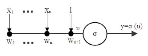
Fig. 1. A perceptron with n inputs and a bias

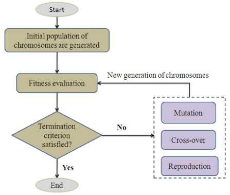
Fig. 2. Schematic diagram of a GA procedure

• B.    Genetic Algorithm

  GAs were introduced by Holland in 1975 as an optimization model, which mimic their behavior from the natural evolution processes, including survival of the fittest, reproduction, crossover, and mutation. A simple

GA cycle consists of three processes. These include selection, genetic operation, and replacement. The population comprises a group of chromosomes. The chromosomes are the candidates for the solution. The fitness evaluation unit determines a fitness value of all chromosomes. The better parent solutions are reproduced, and the next generation of the solutions (children) is generated by applying the crossover and mutation (genetic operators). The crossover operator chooses parents at random and produces children. The mutation operator randomly changes the values of the elements in a string. New generations of solutions are evaluated, and such a GA cycle repeats until a desired termination criterion is obtained [14]. Fig. 2 illustrates a schematic flowchart of GA procedure.

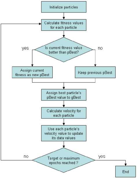
Fig. 3. Flow chart of a PSO algorithm

• C.    Particle Swarm Optimization

This algorithm is an imitation of animal society’s behavior for knowledge processing. The basics of this algorithm comes from two facts; first, the artificial life of animals such as birds and fishes and second evolutionary computations. The computational algorithm of particle swarm optimization (PSO) was developed based on the social behaviors of birds group [15]. The principals of PSO as a population-based optimization method come from large number of birds flying randomly and looking for food together. In this algorithm each particle is the representation of a bird in the natural colony of birds. Any particle has specific velocity, which is influenced by two factors. These factors are dynamically adjusted based on their individual and swarm historical behaviors. All particles save the best position that they have been ever visited during each cycle of the algorithm. This is the first factor that controls the velocity of the particles. In the next cycle of algorithm, the particles starts their movement in the search space, while attracted toward to its previous saved best position (Pbest). The particles share their flying experiences; therefore, their own best position is not only the parameter that the particles save in their memory but also they memorize the best position that has ever been visited by the other particles (Gbest). In the next cycle the particles try to move toward Gbest if the fitness value of this point is better than the fitness value of Pbest. After several cycles the particle are slightly made a convergent to the best position of the search space. Fig. 3 shows the flowchart of the PSO.

• D.    Ant Colony Optimization (ACO)

Ants’ life has attracted the attention of researchers due to its complex social behavior. One of the most amazing behaviors of ants is their ability to find shortest paths from a food source to their nest. Biologists believe that this fact can be possible by splashing special liquid, called pheromones, in their path. The pheromone is an odorous chemical substance that ants can deposit in order to indicate some favorable path for other members of their colony. In fact, the probability for selecting a path is increases when the amount of pheromone increases in the path. Artificial ant colony optimization (ACO) is a relatively new computational intelligent approach, which was initially inspired by the observation of ants. Dorigo et al. [16] have formulated ACO into a meta-heuristics algorithm for solving the optimization problems. A metaheuristics refers to a computer science branch, which selects a computational technique for optimizing a fitness function by improving a candidate solution. The ACO algorithm consists of six main components. These include the particles, a fitness evaluation unit, particle position, search velocity, vaporization, and splashing. Each candidate solution in the problem space is called a particle. In another word, the particle in an artificial ACO plays the role of ants in the real word. The position and search velocity are the characteristics of each particle. The process in which an ACO can find the best solution was explained as below: Firstly, the values of particle position and search velocity for each particle are randomly indicated. The algorithm allows each particle to move through the problem space. Simultaneously, the algorithm saves a record from the particle’s characteristics and evaluates the fitness value of each particle. At the end of this step the particles with higher fitness were selected for the next generation of the colony. Such a procedure happens for the selected in another generation and it continues until the chosen number of generations is achieved. Then, the position and search velocity of particles with the best fitness value were generalized to the environment. In fact, the fitness value shows the amount of pheromones in the path of particles. During the generations, the ACO uses the vaporization and splashing operators to avoid local minimum. Through the vaporization operator, the amount of pheromones is randomly decrease in the paths to avoid the trapping of the algorithm in local minima, while a splashing operator performs inversely. In the searching process of the ACO algorithm, the searching space will reduce gradually as the generation increases. Fig. 4 illustrates a schematic flow chart of ACO algorithm.

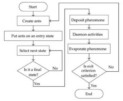
Fig. 4. A representation of ACO algorithm

• IV.    Designing the Optimized Neural Network Models

Weights and biases of the neural network model should be optimized by three optimization techniques including PSO, GA, and AC. The optimization of NN model by optimization techniques is discussed in terms of mathematical concepts below.

If the nth layer of a NN model includes R numbers of inputs and M numbers of neuron, then the weights and biases matrixes of this network are as below.

W ⁿ

Bn

( w 1 ⁿ ) ^T

( w 2 ⁿ ) ^T

(wmn)T bln b'

.b"m _

n n n nT

Where W _m =|_ W _m ,1 , W _m ,2 ,..., W _m , r J and it is vector of weights that connect the m^th neuron of M^th layer to the inputs of that layer. The vector of parameters of this layer can be shown as below.

w 1 ⁿ

X ⁿ

_w 1 _M

b1n bmn

For all layers, the matrixes of weights and biases are defined as the same. The matrixes of all layers form the entire parameters that should be optimized by an optimization algorithm. In simple word, for a network with L layer, the matrix of X variables obtains from below matrix.

X =

X ¹

X ²

Xl

In fact, this matrix is the same with the vector of Eq.(1), while the optimized values of its variables is determined by the optimization technique. To get this goal, first N vectors of location vector (X i ) are randomly generated. The neural network is run so that its parameters (weights and biases) are set based on numerical values of optimization variables. The obtained error of the network is considered as the fitness value of variables vector of the network.

• V.    Developing the Optimized Network Model

The optimized neural network models were trained using a training matrix of conventional well logs and desired responses of NMR log. The correspondence depth of logs and NMR responses were correlated to each other. A brief explanation of data processing is discussed below.

• A.    Selection of Appropriate Inputs

It is necessary to select appropriate well logs for obtaining most accurate intelligent models. The inputs should be sensitive to quantity and type of entrapped fluid in pore spaces. The available well log data were full-suite conventional porosity log of three wells. Each set includes neutron porosity (NPHI), bulk density (RHOB), sonic transit time (DT), effective porosity (PHIE), true formation resistivity (RT), photoelectric factor (PEFZ) and gamma ray log (GR). The corresponding NMR responses are also available for these wells. Studying the previous literatures shows that using all logs reduce the performance of network model due to weak relationship of some logs with the desired outputs; therefore, the cross plot analysis was used to select the most suitable inputs for designing an intelligent model. Table 1 represent the coefficient of determination between the conventional logs and two desired outputs of NMR log. Inputs with higher R2 value have deeper effect on the selected outputs; therefore the arrangement of four logs of neutron porosity (NPHI), bulk density (RHOB), sonic transit time (DT), effective porosity (PHIE) were selected as the most suitable inputs of optimized neural networks. Fig. 5 and Fig. 6 illustrate the cross plots of four selected inputs with FFP and permeability.

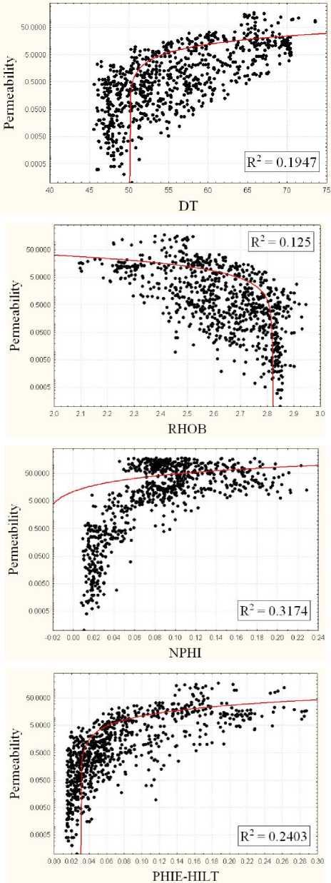
Fig. 5. Crossplots showing relationship between NMR permeability and conventional well log data

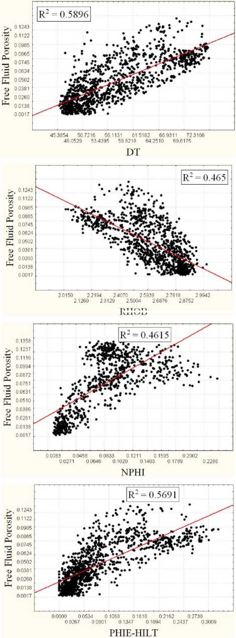
Selecting porosity logs as the most effective inputs of the optimized networks is compatible with petrophysical facts. Porosity logs, such as neutron, density and sonic log, obtain valuable information about the quantity of pore space, which is equivalent to quantity of fluid. Also, the difference of primary and secondary porosity is distinguishable by combination of sonic and neutron logs. Furthermore, PHIE is a good indicator of connected pore spaces; therefore, it is reasonable to see high correlation between the PHIE values and both permeability and free fluid index.

RHOB

Fig. 6. Crossplots showing relationship between NMR free fluid porosity and conventional well log data.

In other hand, gamma ray, true resistivity, and photoelectric factor logs represent information about the distribution of shaly intervals, fluid type, and lithology, respectively. Studying several real case study core data shows no relationship between the numerical variation of these three logs and permeability values. In addition, it seems reasonable to see a weak relationship between resistivity of formation and its FFP and permeability since these two parameters are changed by presence of any type of fluid whether it is water or hydrocarbon, while resistivity log is sensitive to type of fluid. These parameters have negligible contribution in variations of free fluid porosity and permeability.

Table 1. Cross-plot analysis results (R2) for free fluid porosity and permeability

Output Input	FFP	Permeability
RT	0.091	0.023
PHIE-HILT	0.569	0.240
NPHI	0.461	0.317
PEF	0.004	0.026
RHOB	0.465	0.125
GR	0.053	0.048
DT	0.589	0.194

• B.    Preparation of Training Matrix

The available well log data of three wells were used to prepare the training matrix of the optimized network model. The matrix includes 6 columns and 796 rows. Number of rows is equal to number of data points that used. The first 4 rows of the matrix include the numerical value of employed conventional porosity logs, including effective porosity, sonic transmitted, neutron porosity, and bulk density logs. The two last columns are desired outputs of optimized NN model. Preparation of the training matrix is the most crucial step of our research because the PSO algorithm will optimize the weights of objective function just based on the information giving from training matrix. In a simple word, the training matrix is the brain of intelligent system and it has the highest contribution in the accurate performance of trained models for test data. Obviously, the ranges of either inputs or outputs that have not been included in the matrix will be out of responsible for the intelligent model.

Filtering bad-hole interval is another important task that should be noticed. Bad-hole intervals defined as the intervals that the logging instrument failed to detect a reasonable response from the formation. In fact, these points are noise and decrease the performance of intelligent models if they use in training procedure.

Normalization of data is an importance task when working with NN models. This task obviously improves the performance of the model. As shown in Table 2 the tolerance of input and output data is high and this fact affected the results of training procedure. The normalization aims to decrease the negative effect of divergent variables, highlighting important relationships, detecting trends, as well as flattening the distribution of variables to assist the networks in learning the relevant patterns. The input and output data were scaled between the upper and lower bounds of transfer functions of the NN model. In the present study, input and output data were normalized in the range of (-1, 1) and (0, 1), respectively, using the equations 5 and 6.

I

n

= 2(

I -1

min

I max

-

I min

) -1

O n

О - О min

О -О - max     min

Where I n and O n is the normalized value of input and output variable, respectively; I and O denotes the actual value, I min , O min , I max and O max represent the minimum and maximum values of entire data set of the respective input or output, respectively. The input data were normalized in the range of (-1, 1) because the variations of TANSIG function occur in this range. Moreover, it reduces the search space of optimization algorithm. Table 2 represents the range of used data for training the optimized NN. In validation step, the test data should be normalized based on these ranges.

difference is in number of output type and number of neurons in hidden layer. There are four inputs and one output for each model.

D. Extracting the Optimized Weights and Biases

The NN code was introduced to the optimization algorithm to extract its optimized weights and biases. Number of neurons in hidden layer of NN model was adjusted on 11. This value was obtained by a try-and-error procedure in which 25 network models were run and number of neurons was changed from 5 to 30. The mean square error (MSE) for training data was determined for each model. The results show that the minimal MSE is obtained if number of hidden neurons is 11.

After running the optimization algorithm, it takes the NN model as its objective function and tries to optimize it in a way in which the MSE is minimal. Here, the developed MSE function is mathematically introduced. The computational formulation of a three-layered neural network, which contains four nodes in input layer, one node in output layer, and i nodes in hidden layer, is as follow.

NPHI

net Ixl = IWx4 X

RHOB

DT

+ Ib i x l

Table 2. The range of training data used for optimization of weights and biases.

DT	NPHI	RHOB	PHIE-HILT	FFP	K
45.38	0.008	2.09	0.001	0.001	0.001
to	to	to	to	to	to
78.92	0.23	2.94	0.296	0.136	177.

PHIE

out. . =-----—- iX1      i ,    -2 net.

1 + e

-1

C. Implementing the Optimized Network Model

A weak trained neural network model utilizing a good training matrix undoubtedly will fail in validation procedure. In addition, a weak training matrix will conclude to a network performing poor in test step. The combination of a good training matrix and accurate designing of network structure are two crucial parts of developing an intelligent model that guarantees the accurate performance of the model for future applications. In this study, we have tried to cover both of these facts. To design the optimized structure of the NN model, three optimization algorithms were used and the weights and biases of NN model were optimized.

All the necessary codes of this study were written in MATLAB program environment. First, the aforementioned algorithms of GA, PSO, ACO as well as NN were codified in two separate m file . The NN model is the objective function of optimization algorithms and its unknown variable, including weights and biases of neurons, are optimized using a prepared training matrix of conventional porosity logs and NMR responses.

Increasing the number of outputs in a network model causes some complexities and inaccuracies in model construction; therefore in the current research, two separated models were trained for prediction of FFP and K. The structure of the models is the same. The only

Onn = OWi X out xl + bM

Where, IW and OW are matrices of weight factors corresponding to hidden layer and output layer, respectively; Ib and b are matrices of bias values corresponding to hidden layer and output layer; and O NN is estimated value of output. Equation 8 is TANSIG transfer function which is embedded in the nodes of hidden layer. In above formulation, conventional porosity well log data (NPHI, RHOB, DT, and PHIE) are used as inputs, while nuclear magnetic resonance log parameters including free fluid porosity and permeability are used as outputs. To extract the optimum values of weights and biases, following mean square error function was introduced into optimization algorithm.

n

Number of data set in training matrix, initial population of swarms and number of iterations change the time of investigations of optimization algorithm; larger number of aforementioned variables increases the time.

In the last step, the obtained values are substituted in the main formula of NN models, which had been written in Matlab Environment. It is worth mentioning that this

process was done two times; one for permeability and one time for free fluid porosity.

• VI.    Performance of GA-Based Neural Network

Weights and biases of the neural network model were optimized by a genetic algorithm. To get the best results, the training data set was divided into two parts, named training and validation data point including 70 and 30 percent of data set, respectively. First, the model was trained with 70 percent of data and then its performance was evaluated by the remained 30 percent. It leads to the best performance of optimization algorithm. After finding the minimal MSE of the GA, the obtained weights were used for predicting FFP and permeability in testing data points. Fig. 7 illustrates the correlation coefficient of measured and predicted values of FFP and permeability in the test data. The results demonstrate reliable performance of the proposed model. The MSE of the proposed model for FFP and permeability is 3.75% and 4.3 md, respectively. These values are acceptable from the stand point of petroleum engineering in reservoir characterization.

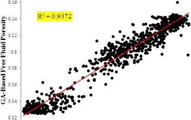
Measured Free Fluid Porosity

(a)

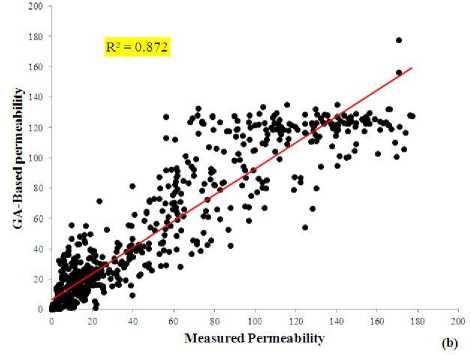
Fig. 7. Crossplots showing the correlation coefficients between measured and predicted results from GA-based neural network for (a) FFP and (b) permeability.

The GA model takes 87.37 second in its best run to find the convergence point of weights and biases. The obtained values of FFP and permeability in the test points were compared to actual values as shown in Fig. 8. The figures show that the proposed model was predicted the trend of increment or reduction in the data. The porous and permeable intervals can be easily distinguished even based on predicted values. This fact shows that the predicted values of FFP and permeability can be used in reservoir modeling with high degree of accuracy.

• VII.    Performance of PSO-Based Neural Network

The same as previous model, the training data were divided into two parts of training and verification. The PSO model was run several times to find its best performance in verification step. Fig. 9 shows the correlation coefficient of measured and predicted values of FFP and permeability using the PSO-based NN. The MSE value of FFP and permeability prediction is 3.32% and 4.1 md, respectively. A comparison between GAbased NN and PSO-based NN shows that PSO-based model performed slightly better. The convergence time of PSO-based model in its best run was 386.89 seconds, which is considerably higher than time of GA-based. The predicted and measured values of FFP and permeability were compared in the testing interval of reservoir (Fig. 10). Similar to previous model, this model was also able to find the trend of data and it is possible to find porous and permeable zones from the non-reservoir intervals, which is the most important parameter of prediction task.

• VIII. Performance of ACO-Based Neural Network

Finally, the ACO-based NN was developed and trained using similar training and validation data. The correlation coefficient of predicted and measured values of FFP and permeability were shown in Fig. 11. The MSE value of ACO-based NN for prediction of FFP and permeability is 5.4% and 7.3 md, respectively. This model is less accurate compared to both of previous models. The convergence time of ACO-based model is 296.83 seconds, which introduces it faster than PSO-based NN but slower than GA-based NN. The predicted values of FFP and permeability were plotted versus depth in the studied well. The same as previous models, ACO-model predicted the trend of data correctly and reliably (Fig. 12).

Figs 8(a), 10(a) and 12(a) show a similarity in prediction task. All Ga-based, PSO-based and ACObased network models overestimate the FFP. It means that for most of test data points the predicted value of FFP is greater that the measured value. A statistical analysis unleashed that the mean value of overestimation is 0.025 (pu), which is negligible from the stand point of petroleum geology for studying the petrophysical parameters of a reservoir rock.

Figs 8(b), 10(b) and 12(b) were also studied in detail. It seems that all optimized neural network models performed accurate in prediction of permeability and the predicted values are close to the actual measured permeability.

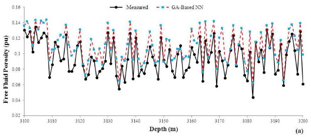
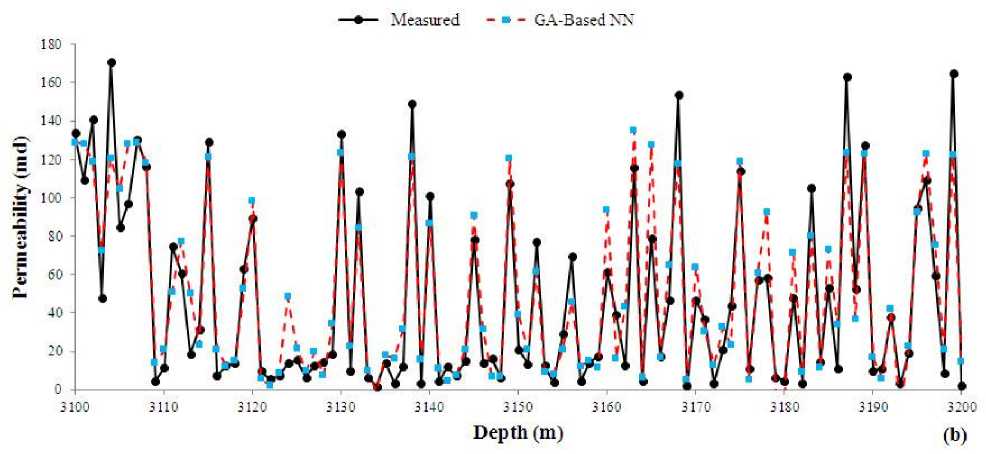
Fig. 8. A comparison between measured and GA-based predicted (a) FFP and (b) permeability versus depth in the test data.

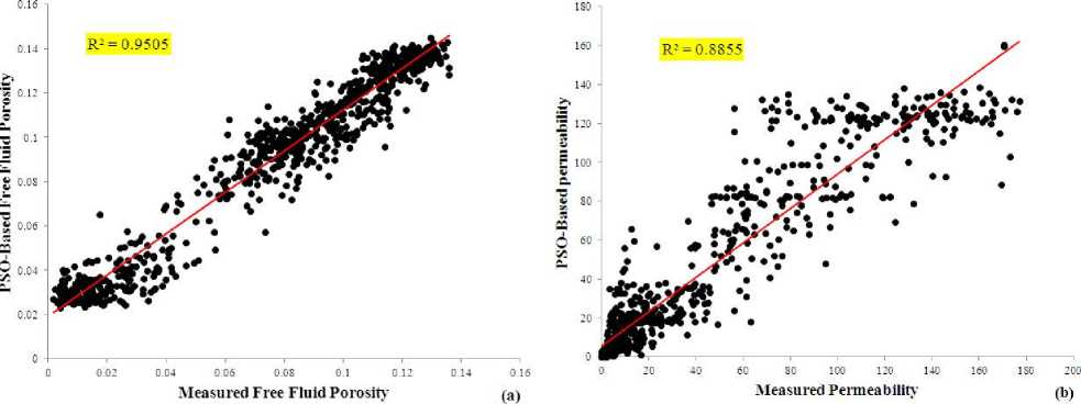
Fig. 9. Crossplots showing the correlation coefficients between measured and predicted results from PSO-based neural network for (a) FFP and (b) permeability.

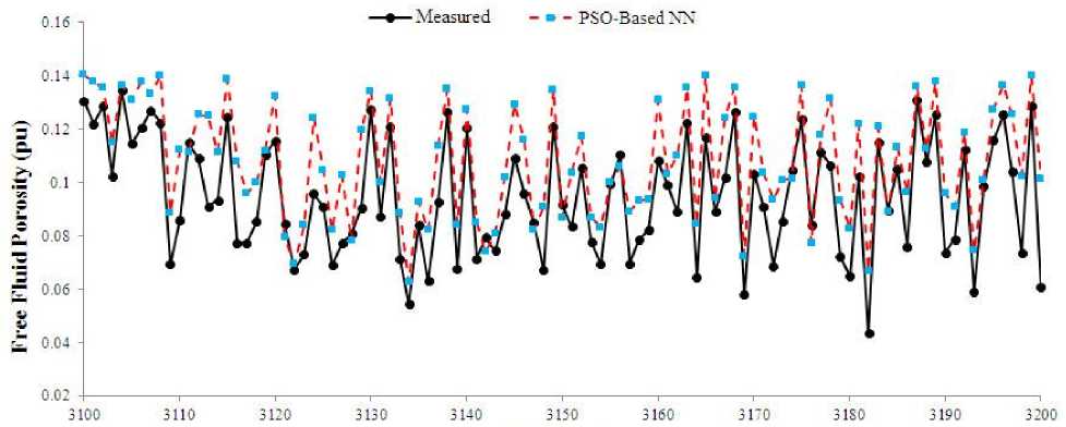
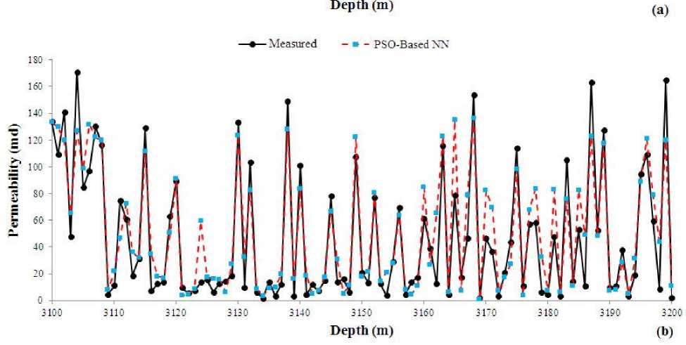
Fig. 10. A comparison between measured and PSO-based predicted (a) FFP and (b) permeability versus depth in the test data.

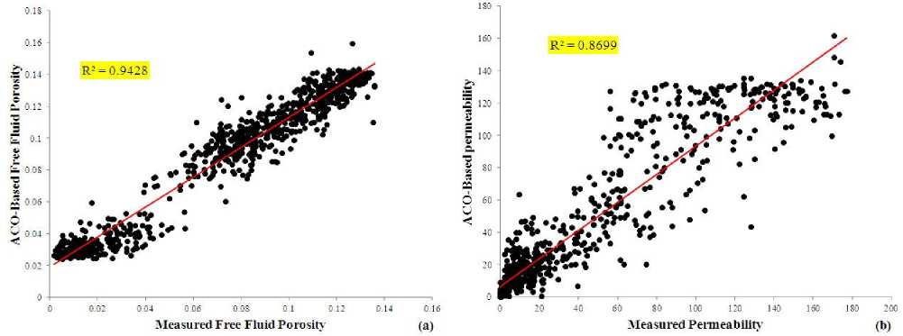
Fig. 11. Crossplots showing the correlation coefficients between measured and predicted results from ACO-based neural network for (a) FFP and (b) permeability.

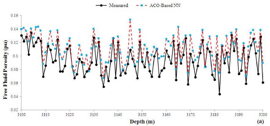
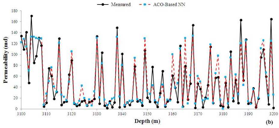
Fig. 12. A comparison between measured and ACO-based predicted (a) FFP and (b) permeability versus depth in the test data.

• IX. Conclusion and Discussion

In the present research, three optimization algorithms, named GA, PSO, and ACO, were used for optimizing the weights and biases of a three layered neural network model. The results show that all of optimization algorithms were performed reliable in finding the NN parameters. Importance of FFP and permeability as two crucial reservoir characteristics motivated the researchers to find the most accurate techniques; therefore, the performance and accuracy of optimization models were investigated in detail. The results uncovered that PSO-based NN model was slightly performed better than GAbased and ACO-based models. From the other hand, the convergence time of GA is considerably smaller than PSO and ACO, which should be noticed when number of training data is high. Considering two features of accuracy and convergence time shows that GA-based model was the best and PSO-based and ACO-based models are in the second and third rank, respectively.

A statistical analysis of predicted values of FFP and permeability uncovers that in all models most of predicted values of FFP are smaller than actual value, while in permeability prediction it is revers. This fact should be considered when the predicted values are employed for modeling tasks. In another word, the developed models based on predicted data will show the reservoir more porous and less permeable than its actual case. The test data are normalized to the range of (-1, 1) using the maximum and minimum data of training matrix before introducing to the optimized trained network and consequently the output of the network is conditioned back to real rang of data using maximum and minimum of training matrix for responses of NMR log. In other words, the estimated output is converted to real values by software before representing in the specific blank part of the interface.

Acknowledgment

The authors would like to appreciate Islamic Azad University of Dashtestan for providing the technical and financial supports of this research. We also extend our warm appreciation to Pars Oil and Gas Company (POGC)

for providing the necessary training matrix of the study. Also, thoughtful, helpful and friendly suggestions of all staffs of Iranian Central Oil Fields Company (ICOFC) during this research are warmly acknowledged.