Application of the Abel equation to cosmological models with and without phantoms

One of the most intriguing concepts in contemporary cosmology is a hypothesis that the dark energy, which governs the observed accelerated expansion of the universe [1], [2], might be phantom in nature. Originally proposed by R. Caldwell in [3], it soon proved to be a fertile ground for mathematical explorations, yielding rather startling results, such as the predictions of Big Rip singularities and the Big Trip phenomena [4], [5], [6], [7], [8], [9] (see also [10]). An interest in the field has been further boosted by the discovery of a “phantom zone crossing” ， which implied that there might exist natural transition from an ordinary cosmological evolution to the characteristically phantom one. However, one of the serious problems that impedes the research in this area lies in the nonlinearity of the Friedman-Robertson-Walker-Lemaitre cosmological equations; while it is not difficult to solve them for the phantom models with a simple equation of state р/с² = wp (where p and p are the density and pressure of a dominant filed of matter, and the constant parameter of state w < -1) [3], it is altogether a different matter to study the general models of a phantom universe filled with a scalar field 0 = 0 ( 。 with some known

* Работа поддержана Министерством науки и высшего образования РФ (договор № 075-02-2023-934).

• ¹    E-mail: vayt 3 7@ gm ail. com

potential V (0), since the equations now take a rather menacing form:

0 = - 3H0 - dV3/"n

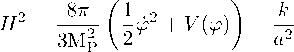
⑴ where к = 0, +1 , —1 correspond to either spatially-flat, closed or open Friedman universe, q = a(t) is a scale factor, H is the Hubble parameter, and V = V(0) is the potential of the scalar field. Note, that (1) is written in the “natural" unit system in which 方=c = 1 and G = M-2. One of interesting (albeit somewhat circumspect) approaches to the problem of solving (1) was the development of a superpotential method, where one postulates the form of a superpotential W = W(0):

爪 =20² + V (0 ) , (2)

which is identified with the density function p, and then reduces the problem to solving a few simple equations [12]; for instance, in the case of a flat universe ( к = 0) all physically meaningful parameters can be derived from the following system:

H = 士 q\/W, ._   1 W ‘

⁰ = 干 3^ TW,

⑶ where a => 0-

This overall rather powerful method contains but a little snag: for many physically important models we do not possess the knowledge of the form W(0) and it is instead the shape of the potential V(0) that is given (e.g., the classical massive field potential V = m02/2). In these situation an additional method is required that would allow to extract the shape of superpotential W(0) from the known function V(0). Such a method for the flat universe models has been developed in [13], [14], in which it has been demonstrated that the problem can be reduced to solving a single first-order O.D.E. called the Abel equation of 1st kind:

*=- 2 仅2 - D 併 - х′y) ,                         ⑷ where 呂=±1, X = V‘/V and the independent variable т = '3寸2a0 [15]. Once the solution of this equation д(т) has been uncovered, the superpotential W is retrieved automatically using the simple relationship:

О2

^W(т) = ^V(т) • о ( д ( ^т)) = ^V(т)       i .                                5

У² ― ¹

This reduction allows to easily study a number of interesting problems such as the problem of the end of inflation for various physically important models [16]. There is, however, something very curious about function 9(y) = у²/(у² — 1). If we take a look at Fig. 1, we can clearly see an inexplicable gap between the values 9 = 0 and 9 = 1. What is going on there?

In order to answer this question, let us recall that 9 is a proportionality factor between W > 0 and V, so it would only satisfy the condition 9 e (0,1) if V > 0 and the kinetic therm:

10² = W — V < 0.                                 (6)

In other words. 0 < 9 < 1 describes the phantom zone!

What shall we do then if we are to account for the phantom zone in our formulas? The first thing we should do is acknowledge that for (6) to hold, 0 must be purely imaginary (the real part of 0 must be

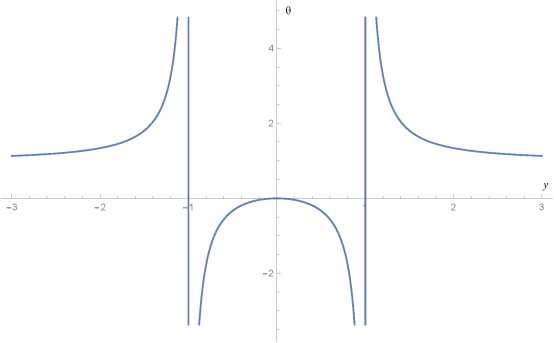
Fig. 1. A graph of function Ө(у ). It can be seen that the range of Ө is (—a, 0] U (1, +x). The lower branch describes the case V < 0 whereas the two upper branches correspond to V >  0.

equal to zero, or by ⑹ either the density p = W or the potential 丿一 or both! — will be complex-valued functions, which is clearly nonphysical). Therefore, one can introduce a new real-valued variable 少 such that:

夕 =I 吵， 少 e R. (7)

Of course, the potential V ( 夕 ) = V ( 2 齢 ) = V ( ① ) must now be real-valued for all ① in the phantom domain, otherwise both the energy density p and the energy pressure 夕 will be unphysically complexvalued. Furthermore, the potential V must be non-negative, otherwise we will end up with a negative energy density ( W < 0 by (6)). So, let's assume that a given potential V satisfies both of these conditions. Then instead of (3) we will have the following system:

H (*= 士 Q ， W (明 ,

= ±

〜 .

1  W ‘

За У^

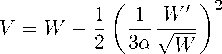
V (9) = W (9) + 2

W ‘ (9)

W(9)

⑻

The systems (3) and (8) are almost identical except for a change in a single sign. However, if we repeat the same calculations as before, taking £ = 3V ^^吵， we would see this sign taking a permanent residence in the resulting calculations [15] - by actually changing the structure of the Abel equation:

弁=|(^2 + 1)(^ —寸 У),

〃£ as well as the relationship between the superpotential W and the scalar field potential V:

W=V • M = V 占.

Note, that the new proportionality factor between the potential and superpotential, 与， is now firmly edged in a previously forbidden zone (0, —1), thus completing the picture as seen in Fig. 2.

Let us now illustrate our approach on a simple example of a scalar field with a constant potential V = const = 0. Since such a potential is always real-valued, regardless of whether the scalar field ф is real or imaginary, this implies that both the classical and phantom dynamics are possible. The Abel equation for a universe from the phantom zone (with imaginary-valued 夕).

У‘ = ± 2 ( У² + 1) ,    / = —13У2а»                           (11)

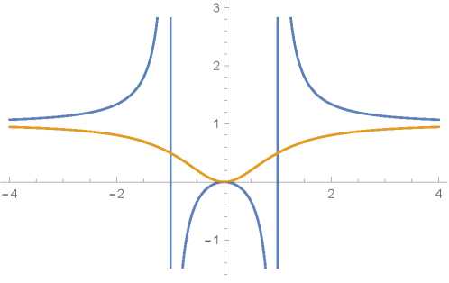
Fig. 2. A graph of both 9(y) (blue) and 9P(y) (orange). As we can see, the classical universe might enter the phantom zone by two routes: either at y т ±s or at y = 0 - both cases corresponding to 0² crossing zero.

Its general solution g and The adjustment factor 0P between W and V are:: x — xo              g2      . 2 Ax — xo\ g = ±tan)，   0 = R=sin         ，

Thus, the superpotential W has the form:

算 о e R

W = 0 • V = Vsin2 (^-^),

which will only be positively defined if V >  0. Knowing the superpotential, it is easy to find H = H ( 算 ):

(x) = 土 avW = 土 avVsin ( 久 .久 ⁰ ).

In order to find H = H(t) we have to use this (real-valued!) equation:

dx dt

±12a ( vW ) ' = ±6a"cos ( ^x - ^x 0 ),

which implies the following relationship between x and t:

sin ( 算 2 算 0 )= 干 tanh ( 3aVV(t — to)).

Hence, the Hubble parameter in this phantom model is H(t) = a^Vtanh ^3a^V(to — t)).

Before we wrap up, let us point out that we can also use the Abel equation to specifically hunt for the potentials that generate the exactly solvable phantom universes. For example, if we choose as a solution of the phantom Abel equation the function g = a/x, a > 0, and plug it into the phantom Abel equation, we can easily extract two possible potentials V(x) that are capable of generating such a solution:

V(x) = ( a² + x² ) e“H2^/(2a) ,     尺 =±1

Note, that these functions are not only well-defined everywhere but they also remain real-valued even if we switch from x to 軒：

V (砌 = ( a² — 18a² /) e^- “ ( 3a 。 ) ² / 。

.

We can now repeat the process we have already discussed: find the superpotential W: W = 0 • V = e"H2/ ( ^2a ) ,

then find the function H = H(x):

H = 土 a" = ± a"/ ( 4a ) ,

etc.