Application Research on High Resolution Radar Target Aggregation

Published Online November 2010 in MECS

Target aggregation need to use data fusion technique. Data fusion is generally defined as the use of techniques that combine data from multiple sources and gather that information in order to achieve inferences, which will be more efficient and potentially more accurate than if they were achieved by means of a single source. Data fusion processes are often categorized as low, intermediate or high, depending on the processing stage at which fusion takes place.[1] Low level fusion, (Data fusion) combines several sources of original data to produce new original data. The expectation is that the fused data are more informative and synthetic than the original inputs.

In high resolution radar system, we usually get a massive amount of original data from observed targets, such as airport scene surveillance radar system. [2][3] Because of the radar system’s real-time requirement, we always need to carry out target aggregation as quickly as possible when multiple original data come form the same source. Airport scene surveillance radar is applied to monitor airplanes, vehicles and some other objects in the air traffic control system. The radar resolution is high, so multiple original data come from the same target. At the same time, there will be some outliers [4] because of noise or communication error. We have to complete target aggregation and outlier removing quickly before target tracking, displaying, etc. In traditional radar data fusion technology, it usually uses statistical methods to compress data and remove outlier, but most of these methods have big calculation amount and cannot comfort to real-time situation. In this paper, we propose a fast target aggregation method based on clustering algorithm to carry out high resolution radar data fusion and satisfy the real-time requirement.

• II.    C LUSTERING ALGORITHM DESCRIPTION

Data clustering is very important in large-scale spatial data preprocessing. Clustering divides the data into different classes (or clusters) by the principle: the data in the same cluster have a high similarity, but the data in different clusters have a great difference. Traditional clustering algorithms can be classified into two main categories: hierarchical algorithm and partitioned algorithm, such as K-means [5], PAM and AGNES [6]. But the spatial data has its own features and traditional clustering methods are not competent for their requirement. So, more and more new clustering algorithms have been proposed in recent researches. CLARANS [7] is based on random search; it can handle large-scale spatial data, and is not sensitive to the order of inputting data, but can only cluster a simple shape, not concave or nested shapes. DBSCAN [8] is a clustering algorithm based on density; it partitions regions with a highly enough density to clusters, and can find any shaped clusters with noise. STING [9] is a grid-based multi-resolution clustering technology, it partitions regions into rectangular space unit, because of the clustering processing is independent of querying, it is efficient. DBCLASD [10] is a density based spatial clustering of applications with noise; comparing with CLARANS, it can find any shaped clusters with high quality; comparing with DBSCAN, it does not need input parameters. Therefore, its efficiency is between CLARANS and DBSCAN. WaveCluster [11] is a multiresolution algorithm; it collects data through a multidimensional grid structure in data space, and then uses wavelet transform to look for dense regions. CLIQUE [12] is an algorithm of combining density-based and girdbased methods; it is very effective for large-scale and high-dimensional spatial database CONQUEST. BIRCH

• [13]    is a comprehensive hierarchical clustering method; it describes clusters with cluster features and cluster feature tree. SOM [14] is a typical presentation of artificial neural networks. FCM [15] is a fuzzy clustering method.

Most of the clustering algorithms’ complexity is nonlinear, and it is not comfort for real-time data processing. We propose a quick target aggregation method based on clustering algorithm in this paper to improve execution efficiency, and to provide a new way to process real-time large-scale data.

• III.    S CENE SURVEILLANCE RADAR SYSTEM

Scene surveillance radar, Secondary surveillance radar (SSR), is a radar system used in air traffic control (ATC), which not only detects and measures the position of aircraft but also requests additional information from the aircraft itself such as its identity and altitude. Unlike primary radar systems, which measure only the range and bearing of targets by detecting reflected radio signals, rather like seeing an object in a beam of light, SSR relies on its targets being equipped with a radar transponder, which replies to each interrogation signal by transmitting its own response containing encoded data. SSR is based on the military identification friend or foe (IFF) technology originally developed during World War II, and the two systems are still compatible today. Monopulse secondary surveillance radar (MSSR), Mode S, TCAS and ADS-B are modern improved versions of SSR.

As shown in Fig.1, scene surveillance radar system mainly includes signal processing and data processing. In order to implement target tracking in real-time, we must complete target aggregation as quickly as possible.

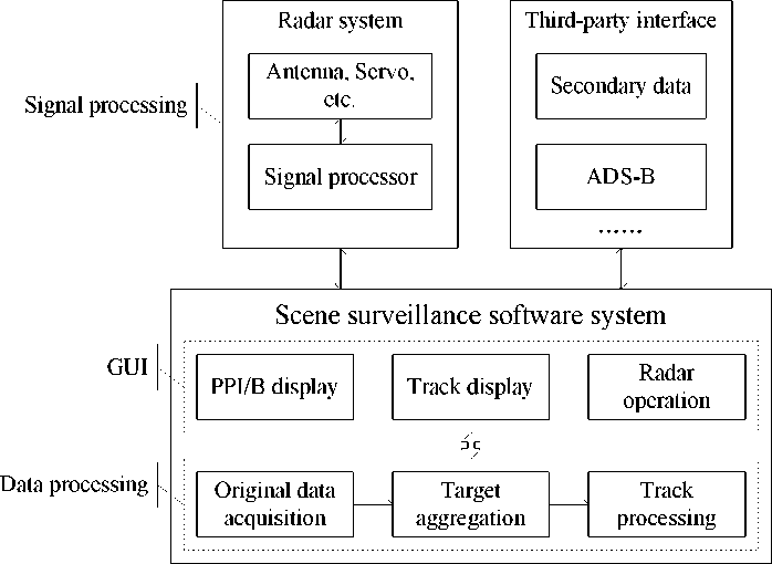
Figure 1. Clustering result of airpot scene surveillance radar data.

• IV.    T ARGAET AGGREGATION METHOD BASED ON C LUSTERING ALGORITHM

The proposed method in this paper is based on clustering algorithm, which only uses simple arithmetical calculation by single dimensional distance. Its idea comes from grid clustering and hierarchical clustering. That is, we divide the original data into subsets in each dimension, and then clustering will be limited to single dimensional calculation. Considering this, the proposed method only needs to scan the original data with linear single dimensional calculation, does not need to compute the multidimensional distance such as Euclidean distance, does not need to search data in whole data space, and does not need to have iterative or recursive call. Therefore, the proposed method’s efficiency is very high.

• A. Definitions and symbol

Firstly, we give some definitions and symbols. Here, we regard each data point as a point p in the m -dimensional data space R ^m . The dataset D is a set of m -dimensional points D = { p 1 , p 2 , ■■■ , p_N } , and N is the number of data points.

Definition 1: data point

In the m -dimensional space R ^m , data point p is defined in (1); pⁱ denotes the i ^th-dimensional component value of data point p .

P = ( P 1 , P 2 , ■■■ , P m )                   (1)

Definition 2: subset

In the m-dimensional space Rm, subset S is defined in (2), {p1, ..., pn} denotes data points set, and {params} denotes the feature parameters of subset S.

S = { { p 1 ,..., P n } ,{ params } }             (2)

Definition 3: single dimensional distance

There are two data-points p a and p b , single dimensional distance is one arithmetical distance of m dimensions; the i ^th-dimensional distance between p a and p b is defined in (3). In addition, the i ^th-dimensional distance threshold is regarded as dist_thⁱ ; the single dimensional distance threshold set is regarded as dist_th .

dist ( Pa , P b ) =| P \, ^- Pb|

dist ( S a , S b ) j = bdr m in ( S b ) j - bdr m ax ( S a ) j |     (9)

Definition 8: neighbor

There are two subsets S a and S b , if their indices meet (10), we call them neighbor in i ^th-dimension.

| idcs¹ ( S _a ) - idcs¹ ( S b )|

< 1

mm

U idcsJ (Sa) I U idcsJ (Sb) * Ф j=i+1                     j=i+1

Definition 4: set-indices

In the subset S , data point p has m indices in every dimension; the i ^th-dimensional index of p is defined in (4). Set-indices are the set of all dimensional indices and defined in (5).

idx' ( p ) = p¹1dist _ th              (4)

idcs ( S ) = \f idx 1 ( p i ), ■■■ , I n idx m ( p i ) ^        (5)

I i = 1                        i = 1                  J

B. Data structure

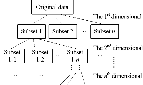
Figure 2. Subset division.

Definition 5: set-borders

In the subset S , the i ^th-dimensional set-border is data points’ i ^th-dimensional minimal value and maximal value. Assume subset S has n group’s indices, the i ^th-dimensional minimal set-border with j index is defined in (6), and the i ^th-dimensional maximal set-border with j index is defined in (7). Set-borders are the set of all dimensional borders and defined in (8).

bdr m in ( S ) j = min ( { P : idx‘ ( P ) = j } )        (6)

bdr_m „( S ) j = max ( { P : idx i ( P ) = j } )       (7)

m

U{(bdrmiin(S)1,bdrmiax(S)1)} i=1

bdrs ( S ) = <■ ■ ■                                r (8)

m

U {( bdr m in ( S ) n , bdr m ax ( S ) n )}

. i = 1

Definition 6: set-density

The number of data points in a subset is named setdensity and regarded as den ( S ). In addition, the setdensity threshold is regarded as den_th .

Definition 7: sets-distance

There are two sorted subsets S a and S b with j index, the i ^th-dimensional sets-distance is the minimal single dimensional distance between S a and S b , and defined in

Mapping to every dimension

For the highest dimension

Repeat n -1 times n : dimension number

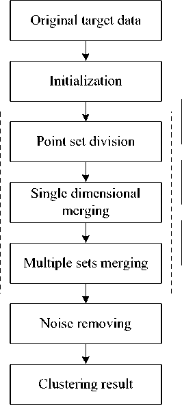
Figure 3. The proposed method flow chart.

In the proposed method, we divide the original data to subsets dimension by dimension as shown in Fig.2, and construct data structure as follows.

dataset. points

It is an n -dimensional matrix of original point set.

dataset. indices

It is an n -dimensional matrix set corresponding original data set.

(1st dimensional index, 2nd dimensional index … dimensional index)

dataset. borders to

nth

It is an n*2 -dimensional matrix set corresponding to original data set.

(1^st dimensional border (min, max), 2^nd dimensional border (min, max) … n ^th dimensional border (min, max))

dataset. merged

It is the mark of a data set whether to be merged by other data set.

C. Algorithm description

• 1)    The algorithm’s whole flow

The flow chart of the proposed method is shown in Fig.3. Firstly, we acquire original data and initialize parameters such as single dimensional distance threshold and set-density threshold, and then divide original data into subsets according to single dimensional distance; finally, carry out clustering also based on single dimensional distance calculation dimension by dimension until get the clustering result.

As shown in table I, in addition to original dataset D , the proposed method algorithm has other two input parameters: one is single dimensional distance threshold set (the threshold can be different in different dimension), another is set-density threshold. Distance threshold set needs to be selected by feature of clusters distance and data points distance in the same cluster, generally, it should be less than the minimal sets-distance between clusters, and greater than the maximal data points distance in the same clusters. Density threshold is related to average number of data points in clusters, and the existence of isolated data points.[16]

TABLE I.

I NITIAL INPUT PARAMETERS

parameter	description
D	spatial data points set
dist_th	single dimensional distance threshold set
den_th	set-density threshold

------------------------------- Single point

* Obtain one set in dimension z

set

Index set from dimension 1 to /-1

Calculate distance of tow sets in dimension z

Merge the right set into the left set

Point set

dimension z ?

Merge sets

Add index set of the right set to index set of the left set

set

Add border set of the right set to border set of left set

set

Delete the right set be merged

Figure 4. Clustering result of airpot scene surveillance radar data.

• 2)    Point set division

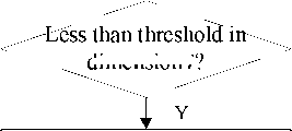
Assume data points have m dimensions; we need to repeat scanning data points m times. In the ith-dimension, we scan all of data points in their parent set, and then divide them into subsets by the ith-dimensional index which is calculated by (4), after data points’ division completed, subsets are sorted by index. After that, we calculate features of subsets. Set-indices are finished before, set-borders are computed by (6), (7) and (8), and set-density is counted.

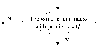
• 3)    Single-dimensional merging

The single-dimensional merging method uses for the highest dimensional subsets merging. Its input includes data subsets divided, distance threshold and the dimension num. We choose two mth-dimensional subsets with same index, if the sets-distance is less than the mth-dimensional distance threshold, they will be merged. In the process, we observe the following rules:

• •    Two m th -dimensional subsets S a and S b with same

index j , if dist m ( S_a , S b ) ^ dist_th _m , merge the subsets;

• ^•    Two m ^th-dimensional subsets S _a and S _b with same index j , if dist m ( S_a , S b ) >  dist_th _m , reserve the subsets.

And its detail process is shown in Fig.4.

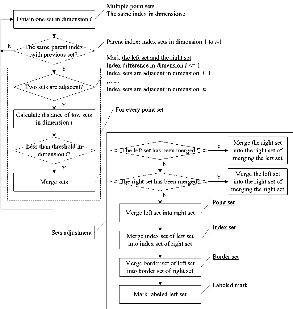
Figure 5. Clustering result of airpot scene surveillance radar data.

• 4)    Multiple sets merging

The multiple sets merging method is for subsets merging after single-dimensional merging. Its input includes sorted subsets, distance threshold and the dimension num. Assume data points have m dimensions; we need to repeat multiple sets merging m-1 times from the (m-1)th dimension to 1st dimension. In the ith-dimension, we choose two adjacent subsets Sa and Sb, if they are neighbors which is computed by (10), just like single-dimensional merging, we judge weather sets- distance is less than the ith-dimensional distance threshold, result is true, we merge the subsets, otherwise, reserve them.

And its detail process is shown in Fig.5.

• 5)    Noise removing

At last, we mark noise or isolated data. If set-density is less than density threshold: 0 <  den ( S ) 5 den _ th , data points in subset S recorded as noise. Then, we can obtain the result of target aggregation.

• D. Complexity analysis

The proposed method scans the original data in each dimension and doesn’t need to calculate Euclidean distance between two data points; all calculations are simple arithmetical calculating by single dimensional distance and set computing by set-indices. Assume m-dimensional spatial dataset D has n data points, and the number of clusters is d. The ith-dimensional subsets division time complexity is O(n), and clustering time complexity is about O(d). The proposed method only needs to scan data points m times without timeconsuming to search the adjacent space. So, its computational complexity is about O(m*n)+O(m*d), usually, d << n, therefore, the algorithm time complexity is approximate to O(m*n).

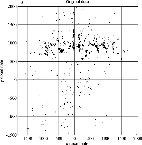
Figure 6. Clustering result of airpot scene surveillance radar data.

• V. E XPERIMENT AND RESULTS

  In this paper, we apply the proposed method to carry out radar target aggregation for high resolution airport scene surveillance radar system. The number of original data is about 3000, and number of effective targets is unknown. Test hardware environment is Intel (R) Core (TM) 2 Duo CPU T8100 @2.10GHz 2.10GHz, memory is 2.00GB; software environment is Microsoft Windows XP Professional, The proposed method is developed by VS.net 2008 C# and Matlab7.01.

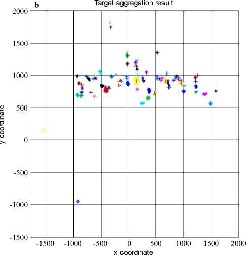
• A.    Radar target aggregation result

  As shown in Fig.6, there are about 3000 original data points come from airport scene surveillance radar system with a lot of noises. (a) Before target aggregation, it includes about 3000 original data points with noise (indeterminate number of true targets); (b) Target aggregation result has approximate 50 clustering results marked by different colors, and the input parameters are: distance threshold = [12 12], density threshold = 5; noise data is removed (number of data points is greater than density threshold).

• B.    Execution efficiency compare

Because of real-time requirement of high resolution airport scene surveillance radar data processing, we are concerned about execution efficiency of algorithm. We compare the proposed method with typical clustering algorithms such as K-means, Hierarchy and DBSCAN as shown In Table 2. Because targets number is unknown in radar data fusion, K-means can not work; Hierarchy and DBSCAN are based on hierarchical method and density method respectively. By comparison, the proposed method is faster than Hierarchy and DBSCAN and it is useful for high resolution radar target aggregation.

TABLE II.

COMPARISON OF EXECUTION EFFICIENCY

Algorithm	Time elapsed (milliseconds)
K-means	k unknown, can not work
Hierarchy	1200
DBSCAN	2700
Proposed	600

VI. C ONCLUSION

For high resolution radar target aggregation, we propose a fast method based on clustering algorithm only using the single dimensional distance calculation. Through m (dimension number) times scanning, the proposed method determines which subset the original data is, and calculates the set-borders and set-density, and then carries out clustering by single dimensional distance threshold and set-density threshold, finally obtains target aggregation result. The proposed method only processes the original data points m times; so, its computational complexity is linear. In addition, all the algorithm’s computing is simple algebraic calculation, the amount of calculation is small, and experimental results confirmed that it is highly efficient. As a highly efficient algorithm, the proposed method has great useful price in practice. However, the method is sensitive to single dimensional distance threshold and the set-density threshold, and it needs to analyze feature of data sets. In the future, we will improve the method’s performance by using adaptive input parameters, parallel computing, etc.

A CKNOWLEDGMENT

The authors would like to thank the anonymous reviewers and editors.