Approximation of solutions to the boundary value problems for the generalized Boussinesq equation

Consider a fluid filtration in a porous layer having finite depth with a free surface u = u ( x,t ). It is necessary to solve initial boundary value problems for the equation [1]

ut   a (u ) xx + utxx, 0 < x < 1 , t > 0,(!)

with boundary conditions

u(0,t) = h(t) > 0, u(1, t) = H(t) > 0, t > 0, a > 0; a = const,(2)

and the following initial condition coordinated with them

u(x, 0) = u0(x) > 0, u0(0) = h(0), u0(1) = H(0)(3)

or with boundary conditions of the second kind

—h o ⁽ t ) , h 1 ( t )

d (ut + au2) x=o = dX (ut + au2) x=1 = which define a fluid flow through the filtration region boundary. The problem (1) - (3) is called the first boundary value problem, and the problem (1), (2), (4) is called the second boundary value problem. The equation (1) is a Sobolev type equation. The initialboundary value problems for analogous equations were investigated in [2-5]. Introduce a function v(x,t) = ut + au2. write the equatkm (1) in the form v — vxx = au2. and invert the operator 1 — Ц2. Then, we have the Cauchy problems for the following integro-differential equations:

ut(x, t) + a • u2(x, t) = a • G G 1(x, £) • u2(£, t)d£ + a • ( — —x)h2 + s^-xH2^) , (Д) sh 1          sh 1    / ut(x, t) + a • u2(x, t)

= a • Gg 2 ( x,£ ) • u ²( £,t ) dy + h о ^Ch(1 — x ) sh 1

Ch x

+ h 1-rr sh 1

with the initial condition (3), where

g i ( x,£ ) = -_i¹ sh 1

sh x • sh(1 — £ ) , 0 < x < £, sh £ • sh(1 — x ) , £ < x <  1 ,

^G 2 ⁽ xS    “.■ I

ch x • ch(1 — £ ) , 0 < x < £, ch £ • ch(1 — x ) ,£ < x <  1

are the Green functions of the corresponding boundary value problems.

If the boundary conditions are stationary, i.e. the functions h ( t ) = h, H ( t ) = H, h ₀( t ) = 0 , h 1 ( t ) = 0 are constants, then the solutions to the considered boundary value problems converge to stationary solutions of the considered boundary value problems [6, 7] uniformly with respect to x as t ^ to.

The stationary solutions have the following form:

• 1)    U 1( x ) = л/( H ² — h 2) x + h ² is the Dupuy parabola,

• 2)    U 2 (x ) = J u ₀( x ) dx is the law of mass conservation in the case of impermeability of 0

the boundary or zero total flow through the boundaries of the filtration region, respectively for the first and second boundary value problems.

In order to obtain approximate solutions and construct profiles of free surfaces of a filtered fluid, we propose to replace the integro-differential equations (5) and (6) with the approximating Riccati equations

u 1 _t + au = aU 2

and

u 2 1 + au 2 — aU 2 ,

respectively. Their solutions that satisfy the initial condition (3) can be found explicitly and have the form:

₍   ) = u o ( x ) + U n • th( a • U n • t )

u n x, “ 1 + uu^x) • th( a • U n • t )

n = 1 , 2 .

Further, the implementation of this method for specific initial conditions is carried out in the MATHCAD. The free surface profiles form one-parameter family of curves in the plane.

Consider some examples of profile construction using the numerical integration of the equations (5) and (6) in comparison with the graphs of solutions to the corresponding equations (7) and (8), where we can observe a difference in the values of the solutions because of the approximations.

Example 1. Consider the first boundary value problem (1) - (3) for h = 1 and H = 4. Calculation formulas for numerical integration of the equation (5) and the coordinates of points of the function (9) graphs have the form, respectively:

u k +i ,i = u ki - « ^ [ u k,i — ^ ( G i i,j • u 1^

A x )1 - shl¹ - i • Д x ) h 2 — sh| i M _{H 2}1 • _д sh 1              sh 1

W ki =

u ₀( i • A x ) + U 1 ,i • th( a • U 1 ,i • k • A t )

where U 1 ,i  =  ^( H ² — h ²) • i • A x + h ² . In this case, if 0 < u ₀( x )   <  U 1 ( x ), then

w k,i < u k ₊₁ ,i < w k ₊₁ ,i and as an approximate value u k ₊₁ ,i

W ki + W k +1 i

. Graphs of approximate solution to the problem (5),

we can take u k ₊₁ ,i = (7) are shown in Fig. 1.

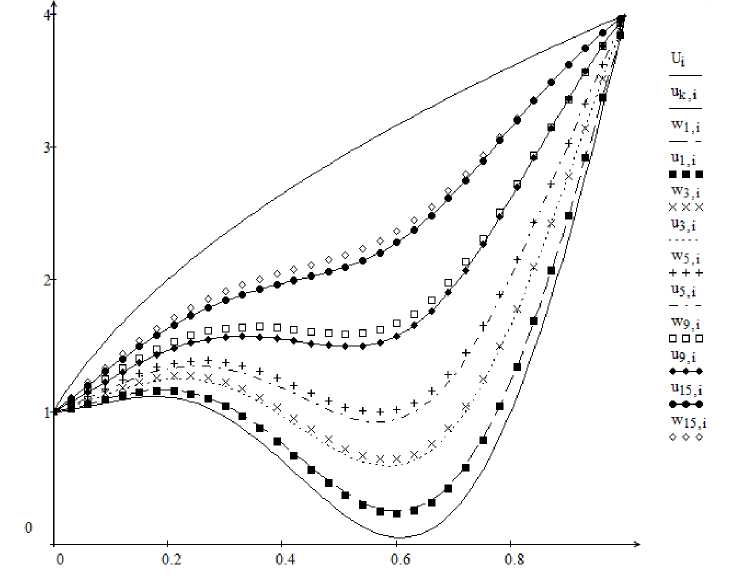
Fig. 1. Graphs of the solutions to the equations (5) (solid lines) and (7) (dashed lines) with the initial condition u ₀( x ) = (3 x — 1)² + sin 2 nx. The upper curve is a graph of the stationary solution, the lower curve is a graph of the initial function u ₀( x ), a = 0 , 8 , A x = 0 , 01 , A t = 0 , 025

Example 2. Consider the second boundary value problem (1), (2), (4). Calculation formulas for numerical integration of the equation (6) have the form:

₂ N            ₂

uk+1 ,i = uki - a uki -     G22i,j • ukj j=0

A x )j   • A t.

Graphs of approximate solution to the problem (6), (8) are shown in Fig. 2.

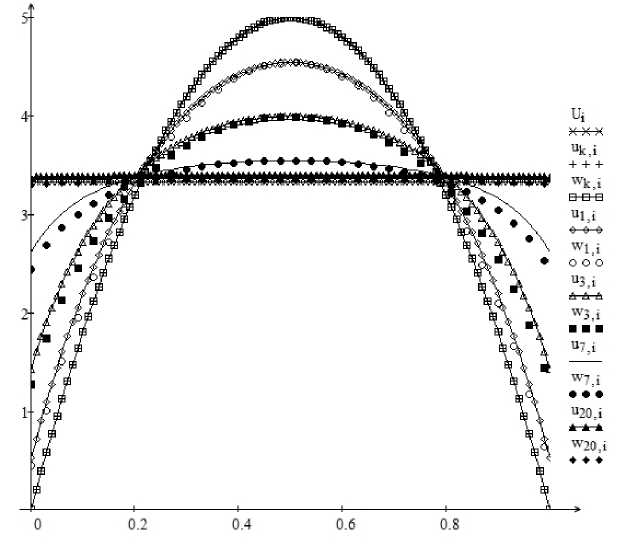
Fig. 2. The graphs of the solutions to the equations (6) and (8) with the initial condition u o( x) = — 20( x2 — x). ar id U2 = J u 0( x) dx = 3, 33.... Ax = 0, 01, At = 0, 05

Acknowledgements. The work was supported by Act 211 Government of the Russian Federation, contract No. 02.A03.21.0011.