Artifacts Removal of EEG Signals By the Application of ICA and Double Density DWT Algorithm

Published Online August 2014 in MECS

Available online at

wave is emitted alone but the conscious state of brain makes a wave more pronounced than other wave for an individual. Five types of waves are stated in [3].

Beta: The rate of change lies in the range of 13 to 30 Hz. It is associated with active thinking, attention and focus. A high of 50 Hz can be seen in state of intense mental activities.

Alpha : The rate of change is in the range of 8 to 13 Hz with 30-50 μV amplitude. The relaxed awareness and the in-attention states are considered to fall in this range. It is considered to be one of the most prominent ranges as beta with a maximum high of 20 Hz is suspected to be Alpha wave. A mindless or empty state of mind falls in alpha category easily distracted by opening of eyes or listening unfamiliar sounds.

Theta: Theta waves lies in 4 to 7 Hz range with an amplitude usually greater than 20 μV. Emotional stress specially frustration or disappointment state of brain produces this category of signals. A deep meditation is state of this category. These waves see a max high of 7 Hz.

Delta: with a variable amplitude and range of 0.5 to 4 Hz signals falls in this category. Deep sleeping state is the corresponding body activity of this state. However this state experiences sound artifact signals produced by the movement of large neck muscles and jaw movement with genuine delta responses. The original signals are produced in the deep brain and are severely attenuated in their path towards skull.

Gamma: Gamma waves lies in the range more than 35 Hz. This state is considered to reflect the mechanism of consciousness.

Many methods have been proposed to remove eye movement and blink artifacts from EEG recordings. As in [4] some of them include simple rejection of contaminated EEG epochs which results in a considerable loss of collected information. Often regression in the time or frequency domain is performed on simultaneous EEG and electrooculography (EOG) recordings to derive parameters characterizing the appearance and spread of EOG artifacts in the EEG channels. However, EOG records also contain brain signals, so regressing out EOG activity inevitably involves subtracting a portion of the relevant EEG signal from each recording as well. Since many noise sources, include muscle noise, electrode noise and line noise, have no clear reference channels, regression methods cannot be used to removed them.

Hence a new and approved method of Independent Component Analysis (ICA) is applied for the detection and removal of artifacts. We have used the Wavelet Denoising techniques along with the ICA for the removal of artifacts from the signals. By ICA we will calculate the mean and variance of the signals and subtract it from base signal to distribute the signal in high and low frequency components. DWT will is then applied to separate both the signals and get the expected outcome.

• 2.    Literature Survey

State of the Art method was introduced initially to eradicate the artifacts from the base signal. The method was made capable to sense the EEG and remove the artifacts simultaneously. The EOG electrodes are placed close to EEG electrodes; they contain a certain amount of brain activity. Thus removing the artifacts cause distortion in EEG signals. Hence further complete methods introduced in this field are summarized in this segment.

Authors in [5] have compared three ICA algorithms i.e. Infomax, SOBI and Fast ICA. These methods allow high degree sensitive automated detection of small non-brain artifacts than the directly applied methods to the scalp channel data. The authors tested all five methods for the performance analysis to detect various types of artifacts by separately optimizing and then applying them to artifact free EEG signals in which manually artifacts of various kinds were added. Except for the muscle artifact detection all the methods involving ICA-decomposed data were superior to raw scalp data.

• [6]    Presents a method for the removal of ocular artifacts in Electro-Encephalogram (EEG) records. The noise source creates the difficulty in the analysis of EEG and clinical information. The authors have proposed the method of Removal of Ocular Artifacts in the EEG through Wavelet Transform without the use of an EOG Reference Channel. The data under consideration is outsourced from a website and sampled at a rate of 128

• 3.    Proposed Methodology

• 3.1    Independent Component Analysis

samples per second. The data is passed through for the identification of spikes and ocular artifacts spike zone. They finally proved that the method provides easy and less complex results with wavelet denoising.

In [7] authors proposed a method for the removal of artifacts from High Density EEG recording during walking and running. They recorded a channel-based artifact template regression procedure and a subsequent spatial filtering approach to remove gait-related movement artifact from EEG signals. First a stride time wrapping for removal of gait-artifact during visual oddball discrimination task and then ICA (isomax algorithm) is applied to parse the channel-based low noise EEG signals into maximally ICs followed by a componentbased template regression. This method reduced spectral power in 1.5 to 8.5 Hz frequency range in condition of walking and running. In walking conditions, gait-related artifact was insubstantial: event-related potentials (ERPs), which were nearly identical to visual oddball discrimination events while standing, were visible before and after applying noise reduction. In the running condition, gait-related artifact severely compromised the EEG signals: stable average ERP time-courses of IC processes were only detectable after artifact removal. These findings show that high density EEG can be used to study brain dynamics during whole body movements and that mechanical artifact from rhythmic gait events may be minimized using a template regression procedure.

In this paper we have used the Independent Component Analysis (ICA) for the segmentation of artifact peaks in the signal. Then the Double Density Wavelet Transform is applied for multi-level transfer of signal data until the reception of significant result.

Consider the two signals x1(t) and x2(t). The x is amplitude of the signals and t is the time frame involved. Let the output signal is s1(t) and s2(t), the function is defined by the equation:

x 1 (t) = a 11 s 1 + a 12 s 2                                                                                                          (1)

x 2 (t) = a 21 s 1 + a 22 s 2                                                                                                          (2)

Where, a₁₁ a₁₂ a₂₁ a₂₂ are some parameters defining the feasibility of the equation. One can determine the values of s1(t) and s2(t) by only the values of x 1 (t) and x 2 (t). This is called as the cocktail party problem. Human mind is able to process and analyze the required sound in the noise. In communication channel the signal is recognized using ICA technique. e. The recently developed technique of Independent Component Analysis (ICA), can be used to estimate the a ij based on the information of their independence, which allows us to separate the two original source signals s 1 (t) and s 2 (t) from their mixtures x 1 (t) and x 2 (t).

ICA Preprocessing: To perform the operations of ICA it is necessary to pre-process the data. Here we discuss the necessary factors involved in this.

Centering: It is the most basic and mandatory step in pre-processing of ICA. The method centers x i.e. subtraction of mean vector m = E{ x } so as to make x a zero-mean variable. Similarly we consider s is also zero-mean. After estimating the mixing matrix A with centered data, we can complete the estimation by adding the mean vector of s back to the centered estimates of s . The mean vector of s is given by A^-1m , where m is the mean that was subtracted in the preprocessing.

Whitening: The second frequent preprocessing step in ICA is de-correlating (and possibly dimensionality reducing), called whitening. In whitening the sensor signal vector x is transformed using formula

у = И^х, s о Е ^уут } = Ц,

Where ∈   , is the -              ( ·  ) whitened vector, and W is × whitening matrix. The purpose of whitening is to transform the observed vectorx linearly so that we obtain a new vector y (which is white) which elements are uncorrelated and their variances are equal to unity. Whitening allows also dimensionality reduction, by projecting of x onto first eigenvectors of the covariancematrix of x.

Whitening is usually realized using the Eigen-value decomposition (EVD) of the covariance matrix {    } ∈   ^× of observed vector x

Rxx = E№ = Ел1\Т ЛУ2 Ex(4)

Here,    ∈    × is the orthogonal matrix of eigenvectors of    =  {   } and ⋀ is the diagonal matrix of its eigenvalues

Лх = й i ад (Л ,,2 ,..,A„)(5)

With positive Eigen values ≥   ≥․․≥   ≥0 . The whitening matrixes can becomputed as

W = Л;1/2 ET

And consequently the whitening operation can be realized using formula

У = Л"х /22Ехх = Wx(7)

Recalling that,   =    , we can find from the above equation that у = Л"Х222E^ Hs = Htos(8)

We can see that whitening transforms the original mixing matrix H into a new one,

H„ = л;222E^ H(9)

Whitening makes it possible to reduce the dimensionality of the whitened vector, by projecting observed vector into first (  ≤  ) eigenvectors corresponding tofirst eigenvalues ,   ,..,  , of the covariance matrix, . Then, the resulting dimension of the matrix W is, × and there is reduction of the size of observed transformed vector y from to .

Output vector of whitening process can be considered as an input to ICA algorithm. The whitened observation vector y is an input to un-mixing (separation)operation s = Ay(10)

Where, A is an original un-mixing matrix. An approximation (reconstruction) of the original observed vector x can be computed as, x =A s,(11)

Where =.

For the set of N patterns x forming as columns the matrix X We can provide the following ICA model

X =

Where 5= [Si , s2,· · · , sn] is the m×N matrix which columns correspond toindependent component vectors S[ = [s^i, S^2,· · · , ] T discovered from the observation vector, xI .Consequently we can find the set S of corresponding independent component vectors as s=      .

Fast ICA Method:

To understand this we use the ICA model given in [8]. A unit is considered to be something that represents processing element. Like for a neuron it has weight W. The weight of several similar other elements considered as w₁ , w_{2 ,} ….., w_n should be determined. In outputs it must be done independent after each iteration in order to avoid convergence of same maxima. The best method is to do analysis one by one.

Algorithms:

• i.    Initialize W[

• ii.    Newton Phase

wt ={ ̃g( w[̃)}-E{д' ( w{ ̃)}Wi(14)

Where g is a function with one of the following form:

gi (y) = tanh(aiy),(15)

g2(y) =yexp(-jy2),(16)

g3(y) =4y3(17)

• iii.    Normalization

Wt = Wi(18)

_‖ Wt ‖

• iv.    De-correlation

Wi =   -∑j^ Wt WjWj(19)

• v.    Normalization like in step iii.

• vi.    Go to step ii. If not converged.

• 3.2    B. Double Density DWT

The statistical independence of unconstrained sources needs to be maximized. The divergences among spatially constrained source sensor projections are bounded to be decremented along with its supporting topographies. The Fast ICA algorithm here extracts the desired components that is a matrix (an array of artifact signals), computed by a corresponding matrix. This saves the critical time of computation, compared to the parallel ICs methods.

The wavelet technique came into existence to overcome the resolution limitations of spectral analysis of Fourier Transform and denoise the corrupted signal. Selesnick et al. [4] introduce the DDWT as the tight-frame equivalent of Daubechies orthonormal wavelet transform; the wavelet filters are of minimal length and satisfy certain important polynomial properties in an oversampled framework. Because the DDWT, at each scale, has twice as many wavelets as the DWT, it achieves slower shift sensitivity than the DWT. The algorithm upgraded in many forms from 1-D, 2-D up to double density complex [9]. The DDWT is implemented on discrete-time signals using the oversampled analysis and synthesis filter bank shown in Figure 4. The frequency responses for the analysis-bank filters are as shown in Figure 1, for a set of filters h⁰, h¹, h² with lengths 7, 7, 5 respectively. The h⁰ filter is a low pass filter, while the h¹ and h² filters are high pass filters with similar frequency magnitude responses. An iterated oversampled filter bank is created by the usual iteration on the low pass branches of the analysis and synthesis banks. Selesnick et al. show that the above DDWT implementation corresponds to a multi resolution analysis with a single scaling function ∅ and two wavelets φ¹, φ² as shown in Figure 1. Observe that the wavelets approximately satisfy the “half-delay” propertyφ¹ (t) =φ² (t-1/2).

The double density DWT is applying the oversampled filter bank on a low-pass sub band signal c(n). In this paper we have used the double density algorithm along with the filter banks.

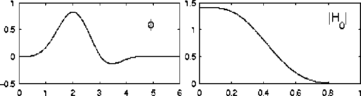
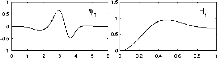
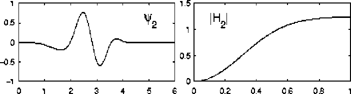
Fig. 1: Left column: basis functions, Right column: frequency responses.

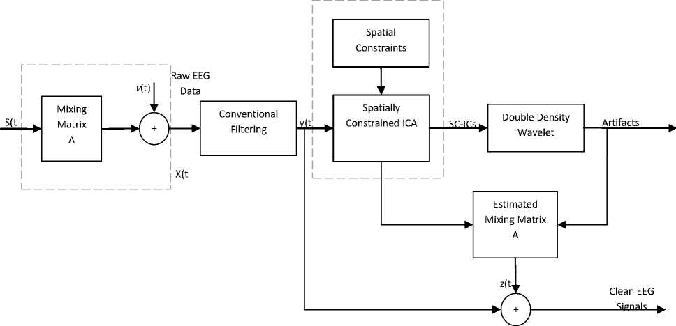
Fig.2: Proposed Flow Diagram of Overall Process of Artifact Removal

The reconstruction condition of filter bank of Figure 3 is derived as follows. We are using basic multi-rate identities we find Y (z), the Z-transform of y(n), in terms of X(z) received as the output matrix of ICA [9].

Y (z) = ^H_o(z)H_og)+H₁(z)H₁gj\x(z) + ¹ - H_o(z)H_o(-^X(-z)                          (20)

Where,

H0 and H1 are the filters.

For perfect reconstruction it is necessary that Y(z) = X(z).

^H(z)H_Q (1) +H - (z)H - (1) = 1

Ho (z)Ho(-j) = 0                                                                                (21)

This can be written as:

H_o (e^iw')H_o(e i ⁽”-^') = 0                                                                              (22)

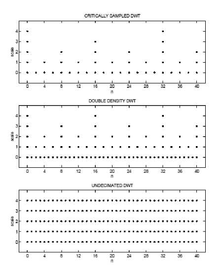
Fig. 3: Idealized time-frequency localization diagrams. The double density DWT gives a denser sampling of the time-frequency plane than the critically sample DWT. But unlike the un-decimated DWT, it maintains the same octave spacing.

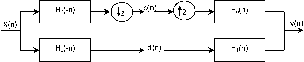
Fig. 4: An oversampled analysis and synthesis filter bank for which perfect reconstruction is impossible with realizable filters.

The H ₀ (e⁷'^w), is discrete Fourier transform of H ₀ (n). The ideal low pass filter is given by:

HQ (ejw)

, 1 W < /22 lQ^ < M < /

satisfies the above equation.

Dual-tree DWT

The double-density dual-tree DWT proposed in this paper is based on concatenating two oversampled DWTs. The filter bank structure corresponding to the double-density dual-tree DWT consists of two oversampled iterated filter banks operating in parallel, similar to the dual-tree DWT. The oversampled filter bank is illustrated in Fig. 5. The iterated oversampled filter bank, corresponding to the implementation of the double- density dual-tree, is illustrated in Fig. 6. We will denote the filters in the first filter bank by ht(n) and the filters in the secondfilterbank by g(п), fori = 0,1,2. Note that in each of thefilterbanks to be considered in this paper, the synthesis filtersare the time-reversed versions of the analysis filters. The goal will be to design the six FIR filters so that they do the following [12].

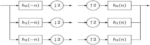
Fig. 5: Oversampled analysis and synthesis filter bank.

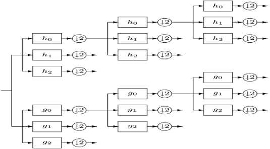
Fig. 6: Iterated filter bank for the double-density dual-tree DWT.

• i.    They satisfy the perfect reconstruction property.

• ii.    The wavelets form two (approximate) Hilbert transform pairs.

• iii.    The wavelets have specified vanishing moments.

• iv.    The filters are of short support.

The -transform of h_t (n) is denoted by H_t (z)

Щ (z) = ZT {h£(n)} = Tnht(n)Z-n

Ht (e1") = D TTTLht()}3 = T^h^e-1™

And G(e¹ " ) is similarly defined. The filters h(n) nnd gt (ri) should satisfy the perfect reconstruction (PR) conditions. From basic multi rate identities, the PR conditions are shown as below:

T=Mz)Ht(lZz) = 2

Zi= о^А^НАМ(27)

And

Z^ о G (z) G AVz) = 2

Z?= о G ^z) G А—1/z) = 0

The scaling and wavelet functions are well-defined implicitly through the dilation and wavelet equations

0„(t) = V2Z„ho(n)0 h(2 t-n)

Фn, i (0 = V2Z„Mn)0 ,(2 t-n)

Фn, 2 (0 = V2Z„ h2 (n)0 h (2 t-n)

Where0_n(t) and/ _g , (t) are defined similarly. The Fourier transforms of the scaling functions and wavelets will be denoted as

Ф „ (w) = r{0_n(t)}, Ф_а(ш) = ^{0₅ (0}

/ ,, Aw) = ^{/ ,, AO}, / , Aw) = Л/ , AO}

The Hilbert transform of a function/(t) will be denoted as H {/(t)}. Following the work by Kingsbury, we want the wavelets to form Hilbert transform pairs

/_a , i (t) = Я{/ 1 At)}                                                                         (35)

/_а , 2 (0=Я{/ 1,2 (0}

Recalling the definition of the Hilbert transform, can be described as:

Vg ,Aw) = {

- Ф ,, Aw),w > 0 jV_h , Aw),w<0

• 4.    Results and Discussion

The proposed methodology was simulated on two data sets. First one was the EEG signals from rats. It is a 5 sec recording of two-channel EEG recording at the right and left frontal cortex of a male adult WAG/Rij rats. Signals were referenced to an electrode placed at the cerebellum and were filtered in the range of 1-100 Hz and digitized at 200 Hz [11]. Example A corresponds to a normal EEG and examples B, C, D and E contain spikewave discharges. The Discrete Wavelet Algorithm and Double Density Algorithm were applied and following results were oriented:

Table 1: PSNR and MSE values on test samples using Discrete Wavelet Algorithm

Samples	PSNR	MSE
Raw_a	37.3613	0.00038510
Raw_b	41.6970	0.00038490
Raw_c	36.1706	0.00038480
Raw_d	38.3893	0.00038450
Raw_e	35.4906	0.00038390

Table 2: PSNR and MSE values on test samples using Double Density Algorithm

Samples	PSNR	MSE
Raw_a	43.7700	0.00038510
Raw_b	46.7562	0.00038500
Raw_c	42.9276	0.00038460
Raw_d	43.9147	0.00038410
Raw_e	42.8613	0.00038390

The second data set is Pattern Visual Evoked Potentials. Each data file is the recording on a different subject in the left occipital electrode (01), with linked earlobes reference. Each data file consists of a several artifact-free trials, with 512 data points (256 pre- and 256 post simulation) stored with sampling frequency of 250 Hz. Data was pre-filtered in the range 0.1-70Hz. All trials correspond to target stimulation with an oddball paradigm [11].

Table 3: PSNR and MSE values on test samples using Discrete Wavelet Algorithm

Samples	PSNR	MSE
Infant_a	9.8288	0.00038508

Table 4: PSNR and MSE values on test samples using Double Density Algorithm

Samples	PSNR	MSE
Infant_a	17.744	0.00038508

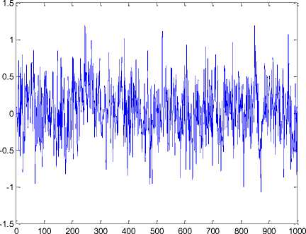
Fig. 7: Input EEG data signal for the test sample Raw_a

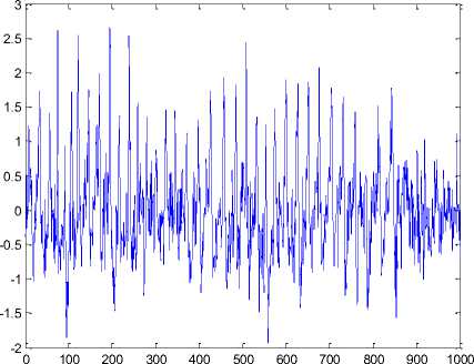
Fig. 8: Input EEG data signal for the test sample Raw_b

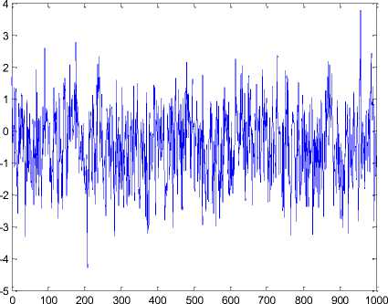
Fig. 9: Output EEG data signal for the test sample Raw_a

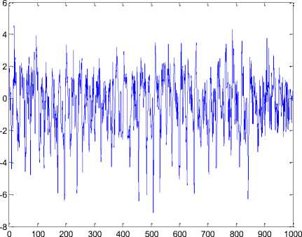
Fig. 10: Output EEG data signal for the test sample Raw_b

• 5.    Conclusion

We studied the artifacts removal of brain signal reports in form of EEG signals. The brain signals obtained are mixed with artifacts at integrated level. The Independent Component Analysis samples the peaks of signals mixed with artifacts and produce segmented outputs. The Discrete Wavelet Transform divides the signal in a multi-level platform until the reception of significant result. The tests were performed on an outsourced EEG data. The Double Density Algorithm was applied in this paper and the comparison was made with DWT. The performance evaluation is measured by PSNR and MSE and finally the comparative analysis of two Data sets is presented in a tabular manner. Hence it is obtained that the method presented was a step superior of the other artifact removal methods.