Artificial Fish School Algorithm Applied in a Combinatorial Optimization Problem

A combinatorial optimization problem P= ( S , f ) can be defined by:

—a set of variables X ={ x 1 , …, x n };

—variable domains D 1 , K , D n ;

—constraints among variables;

—an objective function f to be minimized, where f : D₁ x---x D n ^ IR ⁺ ;The set of all possible feasible assignments is S ={ 5 ={ ( x 1 , v 1 ), ... , ( x „ , v „ )} | v i E D i , s satisfies all the constraints}. S is usually called a search (or solution)space, as each element of the set can be seen as a candidate solution. To solve a combinatorial optimization problem one has to find a solution s ^* ∈ S with minimum objective function value, that is, f ( s ^* ) ≤ f ( 5 ) V 5 e S . 5 * is called a globally optimal solution of ( S , f ) and the set S* c S is called the set of globally optimal solutions.

Combinatorial optimization problems exist widely in the fields of economic management, transportation, communication network and other fields. Its main purpose is to find optimal scheduling, grouping, order or filtering of discrete events. Many combinatorial optimization problems of both practical and theoretical importance are known to be NP-hard, such as the Knapsack problem, the Traveling Salesman Problem (TSP), and Timetabling and Scheduling problems.

Since exact algorithms are not feasible in such cases, heuristics are the main approach to tackle these problems. In the last two decades, swarm intelligence techniques, such as Genetic Algorithm [1], Particle Swarm Optimization (PSO) [1], Bee Colony Optimization (BCO) [2], or Ant Colony Optimization [3], have made some progress in combinatorial optimization problems. They are population-based methods that make use of the global behavior that emerges from the local interaction of individuals with one another and with their environment.

AFSA, which was presented by X. L. Li [4], is a new swarm intelligence optimization method by simulating fish swarm behavior. It is becoming a prospective method because of its good performances in solving traveling salesman problem [5], routing optimization problem [6], complex function optimization problem [7], and so on.

An efficient schedule will improve customer satisfaction, increase port cargo throughout, and enhance port revenues. The BAP involves the determination of berthing times and locations of vessels that are to arrive at a port within a planning horizon, while satisfying a number of spatial and temporal constraints, to optimize operations. Berth planning has been shown to be a NP-hard problem by relating it to the set partitioning problem, the single machine scheduling problem with release dates and the two dimensional cutting stock problem [8]. In recent years, many scholars have studied the BAP using heuristic methods. For example, C. Tong [3] used ant colony optimization to find solutions with good mean costs in a static BAP. K. H. Kim [9] formulated a mixed integer linear programming (MIP) model considering the cost. Experimental results showed that a simulated annealing algorithm obtains solutions that are similar to the optimal solutions found by a MIP model. E. Nishimura [10] developed a heuristic procedure based on GA for determining a dynamic berth assignment to ships in the public berth system, and computational experiments showed that the proposed algorithm is adaptable to real world applications. Many scholars applied their algorithms to different models and used real world data or random numbers in test cases under different computational environments. So it is difficult for us to tell whose algorithm is better.

In this paper, an adaptive AFSA was applied to a BAP. The focus of the paper is on verifying the validity and feasibility of the method and on comparing the convergence performance of the AFSA with that of GA and ACO in a numerical experiment.

The rest of the paper is organized as follows. Section II introduces the model formulation. Section III proposes the adaptive AFSA for the BAP. Section IV presents computational experiments and the final section consists of concluding remarks.

• II.    Problem Formulation

The discussed BAP was a discrete and dynamic berth allocation problem. A number of assumptions were made in the following model as follows:

• a)    Each vessel should be serviced once and exactly once at any berth.

• b)    Vessels should be serviced after the arrival of vessels.

• c)    Vessels should be serviced at any berth with acceptable physical conditions such as water depth and quay length.

• d)    A berth section handled at most one vessel at a time.

The following notations were used in the mathematical model.

• B :    set of berths.

• V : set of vessels.

• i :    i (=1,..., I) e B .

• j :    j (=1,..., J) e V .

b j : the starting time of the service for the j ^th vessel.

A j : the arrival time of the j ^th vessel.

C ij : the service time of the j ^th vessel at the i ^th berth.

X ij : indicated that if the j ^th vessel was serviced at the i ^th berth, X ij was equal to 1, otherwise it was equal to 0.

S_i : the number of vessels at the i ^th berth.

• S : the total number of arrival vessels.

W i : the water depth of the i ^th berth.

D j : the draft of the j ^th vessel including the safety vertical distance for berthing.

P i : the quay length of the i ^th berth.

L j : the length of the j ^th vessel including the horizontal safety length.

Objective: Minimize2 2 (bj - Aj + Cij)Xj(1)

i e B j e V

Subject to: 2Si = S(2)

i e B

2 x, = i(3)

i e B

• b,- a,> 0(4)

(Wi-Dj)X j > 0(5)

(Pi -Lj)Xj> 0(6)

Xj e{0,1}(7)

Equation (1) minimized the total of flow time incurred by vessels. Equation (2) ensured that the total number of arrival vessels was equal to the sum of vessels at berths. Equation (3) ensured that each vessel should be serviced once and exactly once at any berth. Equation (4) ensured that vessels should be serviced after their arrivals. Equation (5) guaranteed that the draft of the jth vessel did not exceed the water depth of the assigned berth. Equation (6) ensured that the length of the jth vessel did not exceed the quay length of the i^th berth [7] [11].

• III. Designing an Adaptive Afsa

• A.    Basic Principle of AFSA

In water areas, following other fish, a fish can always find food at a place where there are a lots of food, hence generally the more food, the more fish. According to this phenomenon, AFSA builds some artificial fish (AF), which search an optimal solution in solution space (the environment in which AF live) by imitating fish swarm behavior. Three basic behaviors of AF are defined as follows [4]:

• a)    Prey: The fish perceives the concentration of food in water to determine the movement by vision or sense and then chooses the tendency.

• b)    Swarm : The fish will assemble in groups naturally in the moving process, which is a kind of living habits in order to guarantee the existence of the colony and avoid dangers.

• c)    Follow : In the moving process of the fish swarm,

when a single fish or several fish find food, the neighborhood partners will trail and reach the food quickly.

The three behaviors’ pseudo-code can be seen in [4].

• B.    Algorithm Design for the BAP

1)    Symbol definition: The following notations were used in the algorithm.

• X : the current status of an artificial fish swarm. X = ( X 1 , X₂ ,..., X_n ), where X_i ( i =1,..., n) represented the current status of the i ^th AF, i.e., the searched solution. It was the berthing sequence assigned to vessels. For example, X i = (1,3;4,2) expressed that vessels S 1 ,S 3 were assigned to berth1 in the order of 1,3; vessels S 2 ,S 4 to berth2 in the order of 4,2.

Y i : the value of function (1) corresponding to X i , i.e., the value of fitness function Y i = f ( X i ).

D_i j : the distance between the i ^th AF and the j ^th AF. It was the number of different elements between X_i and X j . For example, if X i =(1,3;2,5;6,4) and X j =(1,3;6,2;5,4), then D ij =3.

Visual : the visual range of the AF.

N ( X_i , Visual ): set of the visual-neighbors of the i ^th AF.

N ( X i , Visual ) = { X j D j <  Visual } .

• 5 :    congestion degree, 0 <  5 < 1.

FishNum : the population size of an artificial fish swarm.

Maxgen : maximum iterations.

Trynumber : the number of prey iteration.

2)    Behavior description of AF: Let us assume that Xi was the status of the ith AF at present.

• a)    Follow behavior

Step1: For X i , selected the best status X j with the minimum Y j within N ( X_i , Visual ). That is to say, the j ^th AF had the minimum value of objective function among visual-neighbors of the i ^th AF.

Step2: Calculated nf , the number of visual-neighbors of the i ^th AF. If Y j < Y i and nf / FishNum < 5 (there was additional space for other fish), then replaced X i with X j ;

otherwise executed prey behavior. Pseudo code description of the process is presented as follows: Artifical_fish_ follow( )

{

Y j = Min ( f ( X j )), X j ∈ N ( X_i , Visual );

nf = N ( X_i , Visual );

if ( nf / FishNum <  5 and Y< Y i )

then X i = X j ;

else AF-prey ( ) ; end

}

• b)    Prey behavior

Step1: For X i , randomly selected a status X j from visual-neighbors of the i ^th AF.

Step2: If Y j <  Y i , then substituted X j for X i , i.e., X j became the new current status of the i ^th AF; otherwise went to Step1.

If the above operation executed Trynumber times and could not find a better status, then set the last random status as the new current status. Pseudo code description of the process is presented as follows: Artifical_fish_ prey( )

{ for i=0 to trynumber

X j = Random ( N ( X_i , Visual ));

if ( Y j < Y i )

then X i = X j ;

end end

}

• c)    Swarm behavior

Step1: For X i , calculated nf , the number of visualneighbors of the i ^th AF.

Step2: If nf + 0 and nf / FishNum < 5 , determined the central position X c of all artificial fish, in other words, selected the mutual status of the neighborhood partners of X i . Calculated the fitness function Y c = f ( X c ). If Y c <  Y i , which meant that the food concentration of X c was high and the surroundings was not very crowded, then replaced X_i with X_c ; otherwise executed move behavior.

Step3: If nf = 0, executed another behavior. Pseudo code description of the process is presented as follows: Artifical_fish_ swarm( )

{ nf =N(Xi,Visual);

if ( nf + 0 and nf / FishNum < 5 )

then

X c =Center( N ( X_i , Visual ));

Y c = f ( X c );

if Y c <  Y i

• then X i = X c ;

• else AF-move( ) ;

end else

AF-move( ) ;

end

}

• d)    Move behavior

If the optimal solution was not improved in the above optimization progress, generated another status randomly. If the function value of the new status was better than X_i , then adopted it as the current status of the i ^th AF; otherwise executed another behavior.

This behavior could help the solution to escape from local optimum, meanwhile reduced calculation workload and improved algorithm efficiency.

In this paper, four behaviors (follow, prey, swarm and move) were executed in turn, and the latter was used until the former failed. For example, the AF executed follow behavior first, if its status could not be improved, then executed prey behavior.

3)    Constraint strategy: When a vessel moors to a berth, it should meet the requirement of the berth, such as water depth and quay length. The vessel sequence was generated randomly in the algorithm. To exclude infeasible solutions, a large number was appointed to the objective values of infeasible solutions in the process of evaluating solutions. 4)    Stopping Criteria: AFSA is an iterative algorithm, which gradually converges into the global optimal solution. For problems having a known solution, common stopping criterion is maximum iterations. There is another method that checks the variation of the fitness value. If there is very little variation after some iteration, then terminate the calculation. This paper adopted the former. A bulletin board recorded optimal solutions obtained at each iteration and output the best found finally. 5)    Algorithm Procedure: The algorithm procedure of the BAP was described as follows.

Step1: Initialization. Set FishNum , Maxgen , Trynumber , Visual , 5 ; input the expected arrival time and service time of vessels; randomly generated an artificial fish swarm with the population size FishNum , i.e., initialize X = ( X 1 , X 2 , …, X i ,…, X FishNum ). NC = 0.

Step2: For each X i , executed follow behavior; if found a better solution X j , replaced X_i with X j then went to Step7; otherwise went to Step3.

Step3: Rounded Visual x ( 1 - NC / Maxgen ) to the closest integer Visual2 ; if Visual2 >0, went to Step 4 using Visual2 ; otherwise went to Step5.

Step4: For X i , executed prey behavior; if found a better solution X j , replaced X i with X j then went to Step7; otherwise went to Step5.

Step5: For X_i , executed swarm behavior; if found a better solution X j , replaced X_i with X j then went to Step 7; otherwise went to Step6.

Step6: For X i , executed move behavior. If found a better solution X j , replaced X i with X j then went to Step7; otherwise went to Step8.

Step7: NC = NC + 1; updated the optimal solution on the bulletin board.

Step8: If NC = Maxgen , output the current optimal solution, the end; otherwise, went to Step2.

• IV. Computational Experiments

• A.    A Test Case

A test case used in Ref. [7] and [11] was selected to compare the convergence performance of the AFSA with that of GA and ACO. There are two berths in a container terminal. Seven vessels will arrive in a period of time. Assume that the number of quays at every berth is equal and vessels meet constraint (5) and (6) in Part II. Berth1 is idle at 0:00; berth2 is idle at 06:00. The arrival time and the service time of vessels, see Table I.

According to Ref. [7] and [11], there are two optimal solutions: X 1 =(1,5,7,6;3,4,2) and X 2 =(1,5,4;3,2,7,6). The function values of them both are 73[9]. Table II shows partial results obtained by the AFSA.

TABLE I.

V essel I nformation

Vessel name	Information
	Arrival time(hour)	Service time(hour)
Ship1	00:00	12
Ship2	04:00	10
Ship3	06:00	3
Ship4	09:00	8
Ship5	11:00	5
Ship6	18:00	12
Ship7	19:00	4

FishNum leads to the smaller optimal solution of the first generation.

TABLE III.

T he influence of FishNum

Maxgen = 50, Trynumber = 5, Visual = 6 and δ = 0.8
FishNum	5	10	15	20
Time(s)	0.9938	1.0114	1.5968	2.2703
iteration	7	4	2	2

a) FishNum =5

Current best solution 73.runtime:0.86292s

74.6 -

TABLE II.

partial results obtained by the AFSA

Iterations	Current best solution	Objective value
1	1,5,3,7;2,4,6	82
2	1,2,5,7;3,4,6	81
3	1,5,4,7;3,2,6	75
4	1,5,7,2;3,4,6	74
5	1,5,7,6;3,4,2	73

74.4 -

74.2 -

74 -

73.6 -

73.4 -

FishNum=20

Maxgen =50

Ttynumber = 5

Visual = 6

• B.    Parameter Selection Experiments

The method of parameters selection in the algorithm has no strict theoretical basis, the optimal parameters of the algorithm was also a problem need to be solved. So in parameters experiments only one parameter was changed and other parameters are fixed to find its influence on the performance of the algorithm.

The range of parameters in selection experiments was: FishNum = 2~20, Maxgen = 5~50, Trynumber = 5~100, Visual = 2~10 and δ = 0.2~1.0. We have found the random initial value has little effect on convergence performance when parameters do not change. Partial simulation results are shown in Table III~ Table VII .

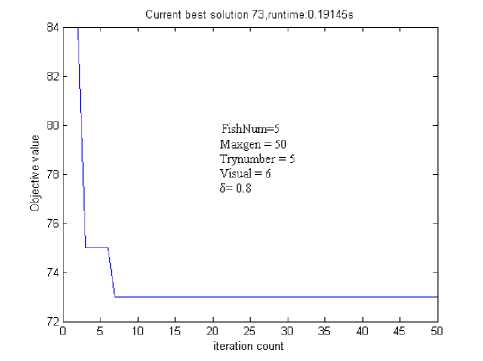
• 1)    The influence of FishNum

73.2 -

With the increase of population size FishNum , iterations with the optimal solution decreases generally and the runtime of the AFSA becomes longer. The increased AF can help the AFSA flee from the local extreme value. For instance, If FishNum < 5, Trynumber < 35, Visual = 6 and δ = 0.8, sometimes the AFSA can not converge after 20 iterations. Fig.1 shows the bigger

73__________________1_________________1_________________1__________________1_________________1__________________1_________________1__________________1_________________1__________________

' 0     5     10    15    20    25    30    35    40    45    50

iteration count

• b) FishNum =20

• Figure1. The influence of FishNum .

• 2)    The influence of Maxgen

When parameters (except Maxgen ) are small, the AFSA usually converges after 20~30 iterations. It means Maxgen must be set as at least 20~30 for obtaining the optimal solution. With the increasing of Maxgen , the runtime of the AFSA becomes longer

TABLE IV.

T he influence of Maxgen

FishNum = 10, Trynumber = 40, Visual = 6 and δ = 0.8
Maxgen	20	40	60	80
Time(s)	0.1701	0.376	0.584	0.957
iteration	5	6	6	3

• 3)    The influence of Trynumber

In general, the increase of Trynumber makes the AFSA converge quickly on condition that FishNum is greater than 4 and Trynumber is greater than 9. But big Trynumber will bring about the increasing of runtime, see Fig.2.

• 4)    The influence of Visual

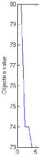
The greater Visual is, the more easily the AFSA finds the global extreme value and converges. The value of Visual must match with the population size of a fish swarm, in general, for 10 artificial fish, only if 3 <  Visual < 7, the AFSA can converge. Fig.3 shows a simulation result when Visual was 2. Besides, the greater Visual will increase runtime generally.

From the above can be concluded, Visual is more important, it reflects the relation of neighborhood fish. It is easier to fall into local extremum using smaller Visual , finally be unable to converge to the global optimal solution. Big Visual will increase searching range, and greatly reduce the algorithm convergence speed; therefore, it is most important that selecting appropriate Visual , where we suggest let Visual be 5.

TABLE V.

T he influence of Trynumber

FishNum = 10, Maxgen = 100, Visual = 6 and δ = 0.8
Trynumber	10	20	30	40
Time(s)	0.651	0.770	0.890	0.9944
iteration	2	4	4	5

TABLE VI.

T he influence of Visual

FishNum = 10, Maxgen = 100, Trynumber = 40 and δ = 0.8
Visual	4	5	7	8
Time(s)	0.843	0.914	not converge	not converge
iteration	6	5	not converge	not converge

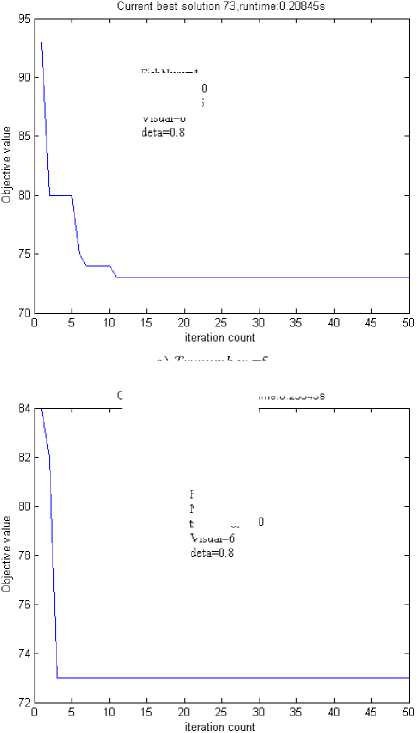
b) Trynumber =20

Figure2. The influence of Trynumber .

Current best solution 89.runtime:0.39435s

FishNum=4 Max_gen=50 trynumber=5 Visual=6

89.6 -

89.4 -

89.2 -

88.6 -

88.2 -

88 L 0

a) Trynumber =5

Current best solution 73.runtime:0.23343s

FishNum=4 Max_gen=50 trynumber= 20 Visual=6

FishNum=l 0

Max_gen=50 ttynumbet—20 Visual=6 Visual=2 deta=0.8

10    15    20    25    30    35    40    45    50

iteration count

Figure3. The influence of Visual

5) The influence of δ

Fig.4 shows the greater the number of FishNum is, the stronger the influence of δ is, the bigger δ leads to the smaller optimal solution of the first generation. A rational value of δ can prevent the AFSA from falling into local extreme value. Besides, we should consider the value of Visual when select the value of δ . Let δ be a large number when Visual is a small number. For example, if Visual = 4, let δ = 1.

FishNum=30 Max_gen=50 ttynumbet—20 Visual=6 Visual=5 deta=0.2

Current best solution 73.runtime: 1.7308s

Parameters: FishNum is 10, Maxgen is 20, Trynumber is 100, Visual

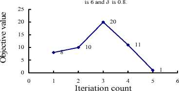
Figure5. Test count and iteration count (for finding X 1 ).

10    15    20    25    30    35    40    45    50

iteration count

a) δ =0.2

Current best solution 73,runtime:1.6732s

75.5 -

75 -

74.5 -

FishNum=30 Ma2_gen=50 ttynumbet^ 20 Visual=6 Visual=5 deta=0.7

74 -

73.5 -

20    25    30    35    40    45    50

iteration count

b) δ =0.7

Figure4. The influence of δ

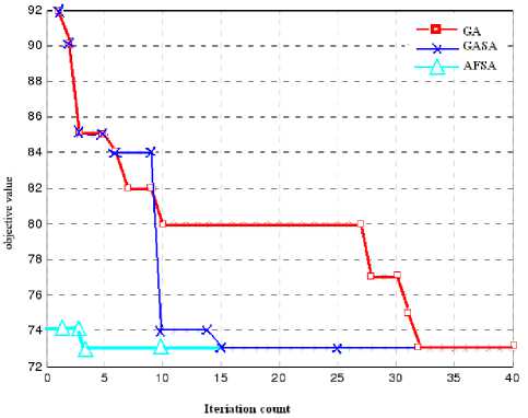
Figure6. Comparing the AFSA with other heuristic methods

TABLE VII.

T he influence of δ

FishNum = 10, Maxgen = 100, Visual = 6 and Trynumber = 40
δ	0.2	0.4	0.6	1
Time(s)	1.014	1.034	1.136	not converge
iteration	3	2	2	not converge

C. Comparing the AFSA with Other Heuristic Methods

Fig.5 shows iteration times for finding X 1 and the number of relative tests (after 50 tests). It clearly shows that the AFSA often converges after about 3 iterations, which are much smaller than that of the GA (32 times in Ref. [7]), hybrid Algorithm of GA and Simulated Annealing (SA), and the ACO (8 times in Ref. [11]). This is to say, the AFSA converges more quickly than the GA and the ACO, see Fig.6. In terms of the computational time, because Ref. [7] and [11] have not introduced their computational environments, we can not compare the runtime, which is about 31~62ms in our tests without plot output (Intel Core 2 Duo E6550, 2.0GB RAM, MatLab) and is about 60ms in Ref. [7].

V. Conclusions

In conclusion, the convergence speed of the AFSA is related to the parameter selection. With rational parameter values, the AFSA can approach and obtain the optimal or sub-optimal solution. In order to make AFSA more useful in a BAP and to compare its performance with that of other heuristic methods, we improved original AFSA for the BAP. The experimental results show that the model is capable of allocating berths efficiently and the algorithm can lead to satisfactory results in allowable CPU time. The AFSA can adjust the searching range adaptively by four search behaviors. The computational time and the quality of solutions depend on parameter selection. Optimizing parameters could further improve convergence performance. The improved AFSA converges more quickly than the GA in Ref. [7] and the ACO in Ref. [11]. The algorithm has improved the efficiency of the berth scheduling and has some practical significance.

Although the AFSA provided a new idea to solve the BAP, in practice, the schedule of quay cranes is considered in the BAP sometimes, because the service time of a vessel varies with the number of cranes assigned to it. So the issue of crane scheduling will be incorporated into the next model for further study. In addition, there are some other objectives should be considered, such as the cost, the traffic, etc.

Acknowledgment

This research was supported in part by the project fund of the Hubei Province key laboratory of mechanical transmission and manufacturing engineering Wuhan University of Science and Technology (2007A08).