Auditory Model Identification Using REVCOR Method

Author: Lamia Bouafif, Noureddine Ellouze
Journal: International Journal of Intelligent Systems and Applications(IJISA) @ijisa
Article in issue: 9 vol.6, 2014.
Free access
Auditory models are very useful in many applications such as speech coding and compression, cochlea prosthesis, and audio watermarking. In this paper we will develop a new auditory model based on the REVCOR method. This technique is based on the estimation of the impulse response of a suitable filter characterizing the auditory neuron and the cochlea. The first step of our study is focused on the development of a mathematical model based on the gammachirp system. This model is then programmed, implemented and simulated under Matlab. The obtained results are compared with the experimental values (REVCOR experiments) for the validation and a better optimization of the model parameters. Two objective criteria are used in order to optimize the audio model estimation which are the SNR (signal to noise ratio) and the MQE (mean quadratic error). The simulation results demonstrated that for the auditory model, only a reduced number of channels are excited (from 3 to 6). This result is very interesting for auditory implants because only significant channels will be stimulated. Besides, this simplifies the electronic implementation and medical intervention.
Auditory Filter, Gammashirp, SNR, MQE, Revcor, Channel Stimulation
Short address: https://sciup.org/15010599
IDR: 15010599
Text of the scientific article Auditory Model Identification Using REVCOR Method
Published Online August 2014 in MECS
The study of the auditory models was developed by psychoacoustics and biomedicine specialists especially in the field of the cochlea and auditory implants.
Several auditory models have been developed and implemented on ship such as the DSAM of the HUTear, the Earlab data viewer application which was developed by the hearing research Lab at Boston University and the Auditory Toolbox [1].The DSAM library is programmed in C. It simulates many models such as the Gammatone auditory filter, Meddis [2], and the auditory imagery Model (AIM) of Patterson. In addition of the Gammatone filter, the library contains the auditory model of Lyon [3] and Seneff[4]. Besides, we find in the several references many others models of auditory filters such as those of Revcor[5], Boer[6], Houtgast[7], Patterson an Roex [8].
In this study, we will develop a new auditory model based on the gammachirp filterbank analysis. At the first step, two auditory models will be presented essentially the analytic model and the REVCOR experimental model. In order to validate this model and to optimize its parameters, a comparison between the experimental and the simulated responses will be conducted. Finally, we will apply our strategy on several database speeches in order to determine the hearing bands containing the maximum information and to deduce the appropriate stimulation channels.
-
II. The Revcor Principle
The technique of REVCOR or "Reversed Correlation" is a method used by neurophysiologists to estimate the response of an auditory neuron [7]. This technique, initiated by Boer and Jongh, is based on the fact that when the filter input is a white noise, the correlation function between the filter input and output is its impulse response [9], [10].
The following expression presents the impulse response filter under the form of a pulse trains noted S(t) :
N
S (t)=£ 5(t - ti) i=1
t i : represents the releasing times of the electric impulses.
The cross-correlation or REVCOR of the signal X(t) with the output filter is noted Ф xs (t):
+X
фз (т) = J X(t)S(t + t)dt (2)
-X
+x
»xs(т) = J X(t)[(X * h)(t + т)] dt
-X
+x +X
= J J X (t) X (t + т -1') h (t') dt' dt
-X -X
with:
h(t) represents the filter impulse response.
Changing the order of integration, we make appear the cross-correlation function:
+X
Фxs (t) =JФxx (t - t')h(t')dt' (4)
-X
If the input signal is a white noise, then we obtain the following autocorrelation function:
ф хх ( т ) = N 0 ^ ( т ) ф хх ( т ) = N о З ( т ) (5)
N o : is the spectral density of the noise.
Like this, we obtain the following function:
ф XS ( т ) = N 0 h ( т )
-
III. Experimentation
The validation of this method was performed by the experiment of Fig.1 applied on a cat: the result is the impulse response REVCOR.
The experiments values are extracted from Carney Database developed by the EARLAB laboratory of Wisconsin University [9].
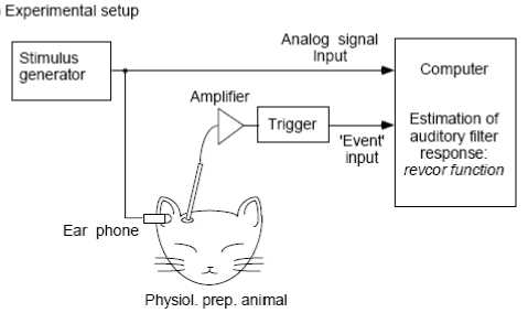
Fig. 1. REVCOR experimentation
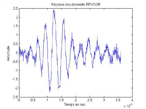
An example of the impulse response recorded by the technical Revcor is given by Fig.2.
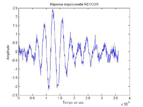
Fig. 2. Revcor impulse response measured on a nerve of an auditory fiber of a cat with 3000 Hz
-
IV. Gammachirp And Gammatone Model
-
A. Theorical auditory model
The gammatone model has been proposed to the first time by Johannesma. This temporal model was deduced from the impulse responses measured from the electric impulses of the nervous fibres of the internal ear [4]. Irino and Patterson proposed a new model of the auditory filter called gammachirp, taking into account rectangular auditory bands [11]. The impulse response of the gammachirp filter is given by the following expression [12]:
g c ( t ) = at n - 1 exp( - 2 n bERB(f r ) t )
with:
n : filter order, fr : is the modulation frequency of the gamma function, a: is the carrier normalization parameter, c : is the asymmetry coefficient of the filter, ф : is the initial phase bERB: is filter envelope,
ERB : represents the equivalent rectangular band given by [7], [2]:
ERB (fr) = 24,7 + 0,108 . fr (8)
The ERB of each gammashirp filter is calculated in function of the central frequency (fr) according to Fletcher [3]. If we use the formula of Glasberg and Moore [2] and if we suppose that the signal band is between fH and fL with a filter recovery ratio (v) hence, the number of filters (N) is selected like this [13]:
N = 9.26 In v
.fH + 228.7 f L + 228.7
However, the central frequencies (fr) can be deduced by the expression [14]:
vn fr = - 228.7 + (fH + 228.7)e 9.26 (10)
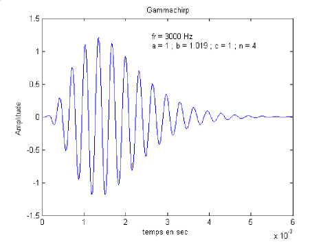
An example of the temporal response of the Gammachirp filter is illustrated by the Fig.3.
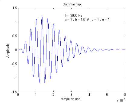
Fig. 3. Temporal answer of a Gammachirp function centred on 3000 Hz, with a =1, b=1.019, c=1, n=4 and f=0.
The Frequency response of the filter bank Gammachirp model [15] is illustrated by Fig.4. It shows exactly the ear anatomy with multiple bands. The envelope curve represents the hearing threshold. The channels number, the bandwidth and the central frequencies of each channel are illustrated in table 1. They are computed according the last expressions (8), (9) and (10).
This kind of filter represents a good approximation of the inner ear and especially the cochlea and gives a good estimation of pitch and formants by using the psycho-acoustical experiences [7].
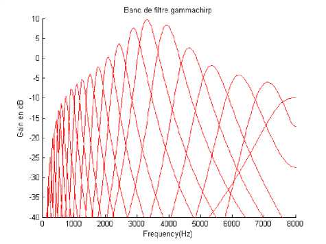
Fig. 4. Frequency response of the Gammachirp model
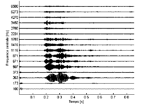
Fig. 5. Temporal representation of the gammachirp filterbank outputs for the vowel /a/ (N=16 channels)
The following table represents an example of a filter bank decomposition with 25 GFB critical bands.
Table 1. Normalization of critical bands in Bark scale
|
Central frequency |
bandwidth |
Channel N° |
|
100 |
100 |
1 |
|
150 |
100 |
2 |
|
250 |
100 |
3 |
|
340 |
100 |
4 |
|
450 |
110 |
5 |
|
570 |
120 |
6 |
|
700 |
140 |
7 |
|
840 |
150 |
8 |
|
1000 |
160 |
9 |
|
1175 |
190 |
10 |
|
1370 |
210 |
11 |
|
1600 |
240 |
12 |
|
1850 |
280 |
13 |
|
2150 |
320 |
14 |
|
2500 |
380 |
15 |
|
2900 |
450 |
16 |
|
3400 |
550 |
17 |
|
4000 |
700 |
18 |
|
4800 |
900 |
19 |
|
5800 |
1100 |
20 |
|
7000 |
1300 |
21 |
|
8500 |
1800 |
22 |
|
10500 |
2500 |
23 |
|
13500 |
3500 |
24 |
|
19500 |
3500 |
25 |
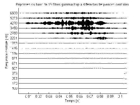
Fig. 6. Temporal representation of the gammachirp filterbank outputs for the consonant /sh/ (N=16 channels)
Temps [sj
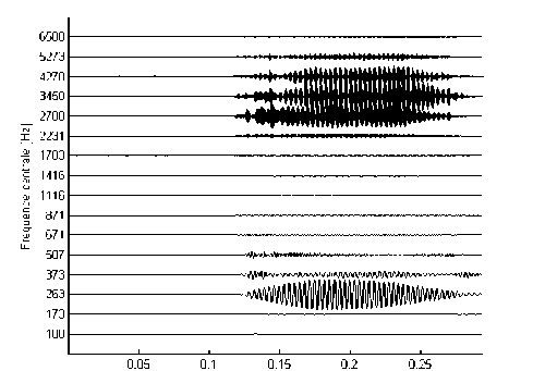
Fig. 7. Temporal representation of the gammachirp filterbank outputs for the vowel /i/ (N=16 channels)
Temps [s]
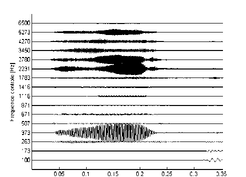
Fig. 8. Temporal representation of the gammachirp filterbank outputs for the vowel /u/ (N=16 channels)
(c) Comparison between simulation and experimental results
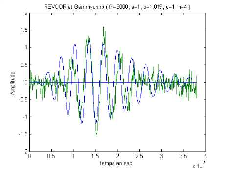
Fig. 9. Superposition of the Revcor impulse response of an auditory nerve with Fr frequency = 3000 Hz and the Gammachirp function centred on Fr, with a =1, b=1.019, c=1, n=4
Fig.5, 6, 7 and 8 illustrate a simulation of the temporal responses of the 16 Gammashirp filter channels for the three vowel audio input signal (/a/,/u/, /i/) and an unvoiced audio signal (consonant (/sh/) .
(a): experimental response
-
B. Comparison of Revcor and Gammachirp results
In order to validate the Gammashirp model and to optimize its parameters, a comparison between the REVCOR experimental results and the simulated responses of the analytic model is presented. The validation is conducted by computing at every time the mean quadratic error MQE and the SNR (signal to noise ratio) in order to optimize the recover parameters of the Gammachirp function that gives the minimal value of MQE. Fig.8 represents the superposition of Revcor and the simulated Gammachirp model.
-
C. Simulation results and parameter optimization
Tables 2 and 3 give the MQE values between the Revcor impulse response| of an auditory nerve and the gammachirp auditory model with the same central frequency.
(b) Gammachirp model response
Table 2. parameter optimization
|
Fr (Hz) |
a |
B |
c |
n |
MQE |
|
< |
2 |
3 |
1 |
4 |
17.35 |
|
1 |
3 |
1 |
4 |
5.29 |
|
|
1 |
8 |
3 |
4 |
1.44 |
|
|
1 |
8 |
5 |
4 |
1.45 |
|
|
1 |
8 |
1 |
4 |
1.45 |
|
|
1016 < |
1 |
3 |
3 |
4 |
0.137 |
|
2 |
3 |
3 |
4 |
0.485 |
|
|
1 |
4 |
3 |
4 |
0.033 |
|
|
1 |
7 |
3 |
4 |
0.018 |
|
|
1 |
8 |
3 |
4 |
0.017 |
|
|
1 |
8 |
3 |
5 |
0.018 |
|
|
1 |
3 |
1 |
4 |
0.132 |
|
|
1523 |
1 |
1 |
1 |
4 |
17.72 |
|
2 |
1 |
1 |
4 |
70.91 |
|
|
2 |
3 |
1 |
4 |
0.052 |
|
|
1 |
3 |
1 |
4 |
0.019 |
|
|
2 |
3 |
3 |
4 |
0.050 |
|
c |
8 |
3 |
4 |
0.008 |
|
|
1 |
8 |
1 |
4 |
0.0081 |
|
|
2035 |
1 |
3 |
2 |
4 |
0.5197 |
|
3 |
3 |
1 |
5 |
0.5217 |
|
|
1 |
2 |
1 |
4 |
0.5084 |
|
|
1 |
3 |
1 |
4 |
0.5108 |
|
|
c |
2 |
1.019 |
1 |
4 |
0.5094 |
|
1 |
8 |
3 |
4 |
0.5217 |
|
|
3 |
1.019 |
1 |
4 |
0.5062 |
|
|
2500 |
1 |
1 |
1 |
4 |
1.0305 |
|
2 |
1 |
1 |
4 |
4.1163 |
|
|
1 |
2 |
1 |
4 |
0.0094 |
|
|
1 |
8 |
1 |
4 |
0.0012 |
|
|
1 |
8 |
3 |
4 |
||
|
1 |
3 |
3 |
4 |
0.0016 |
|
|
3000 |
1 |
1 |
1 |
4 |
0.5005 |
|
1 |
1.019 |
1 |
4 |
0.4674 |
|
|
1 |
8 |
3 |
4 |
0.2431 |
|
|
1 |
1.02 |
1 |
4 |
0.4658 |
|
|
1 |
__0------ |
—I---- |
-^4----- |
--0-0/100 |
|
|
< |
|||||
|
1 |
3 |
1 |
4 |
0.2437 |
|
|
1 |
3 |
2 |
4 |
0.2445 |
|
|
1 |
5 |
1 |
4 |
6.9351 10-5 |
||
|
1 |
8 |
3 |
4 |
6.9104 10-5 |
||
|
1 |
8 |
3 |
5 |
6.9010 10-5 |
||
|
2 |
8 |
3 |
5 |
6.9013 10-5 |
||
|
1 |
1 |
8 |
4 |
0.0116 |
||
|
6406 |
1 |
3 |
1 |
4 |
7.0485 10-4 |
|
|
1 |
3 |
2 |
4 |
7.0836 10-4 |
||
|
1 |
3 |
1 |
5 |
7.0796 10-4 |
||
|
1 |
3 |
8 |
4 |
7.0813 10-4 |
||
|
2 |
3 |
1 |
4 |
7.0365 10-4 |
||
|
5 |
3 |
1 |
4 |
7.1152 10-4—J |
||
|
1 |
8 |
1 |
4 |
7.0813 10-4 |
||
|
1 |
8 |
3 |
4 |
7.0813 10-4 |
The values in bold correspond to the optimized parameters as they conduct to the minimal errors MQE. We can conclude that for the GBF filter, the optimal parameters of the auditory model are:
a=1 л
B=8
C=3 □
N=4
Note that every (Fr) frequency corresponds to the Glasberg band of the GFB filter. Besides, according to the last Fig. 5, 6, 7 and 8, we can deduce that for the auditory model, only a reduced number of channels are excited. For example, for the analysed vowels, there are 3 to 5 (from 16 or 32) significant channels which are stimulated.
This result is very interesting for auditory prosthesis and cochlea implants because it simplifies the electronic implementation.
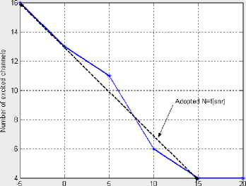
D. Noise effect (SNR)
To investigate the robustness of the auditory model, we calculated the number and the order of channels which will be excited in noisy environments. For example, table 4 and fig. 10 represent the number of excited channels (No) according to SNR. We can easily observe that the variation follows the following law:
No = N max - 0.6 (SNR+5)
Table 3. Parameter optimization
|
Fr (Hz) |
a |
B |
c |
n |
MQE |
|
3593 c |
1 |
3 |
3 |
4 |
2.3267 10-4 |
|
2 |
3 |
3 |
4 |
2.6708 10-4 |
|
|
1 |
3 |
1 |
4 |
2.14469 10-4 |
|
|
1 |
8 |
3 |
4 |
1.8913 10-4 |
|
|
—7+— |
-4 |
||||
|
2 |
8 |
3 |
1.8931 10 |
||
|
1 |
7 |
3 |
4 |
1.8915 10-4 |
|
|
3789 |
1 |
1 |
1 |
4 |
0.970 |
|
1 |
2 |
1 |
4 |
0.901 |
|
|
1 |
4 |
1 |
4 |
0.900 |
|
|
1 |
3 |
1 |
4 |
0.901 |
|
|
1 |
2---- |
-4— |
|||
|
1 |
3 |
2 |
4 |
0.902 |
|
|
1 |
3 |
3 |
4 |
0.901 |
|
|
1 |
1 |
1 |
4 |
0.970 |
|
|
4219 |
1 |
3 |
3 |
4 |
7.4375 10-5 |
|
1 |
1 |
1 |
4 |
0.0345 |
|
|
2 |
1 |
1 |
4 |
0.1375 |
|
|
1 |
5 |
3 |
4 |
5.7165 10-5 |
|
|
1 |
8 |
3 |
4 |
5.6442 10-5 |
|
|
1 |
7 |
3 |
4 |
5.6524 10-5 |
|
|
4961 |
1 |
1 |
1 |
4 |
0.0117 |
|
1 |
2 |
1 |
4 |
9.4297 10-5 |
|
Table 4. The noise effect on MQE and stimulated channels
|
SNR in dB |
Number of stimulated channels |
Mean Quadratic error: MQE |
Maximum number of channels |
|
15 |
4 |
0,0021 |
22 |
|
10 |
6 |
0,0037 |
22 |
|
5 |
11 |
0,0078 |
22 |
|
0 |
13 |
0,0095 |
22 |
|
-5 |
16 |
0,0110 |
22 |
effect of the noise on tne number of stimuli
SNR of input signal in dB
Fig. 10. Number of excited channels in function of SNR
Expression (11) shows that with very noisy signals (SNR <-5dB), all channels (n=Nmax) must be stimulated
for high speech intelligibility and acceptable recognition rates. Generally, for each decrease of 5 dB, SNR must be compensated by increasing 3 additional stimulated channels. This result is very important because it solves the problem of performance degradation of the cochlear implant environment and gives priority to electrical stimulation compared to acoustic stimulation.
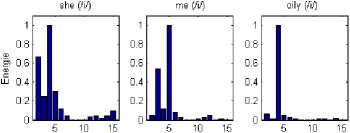
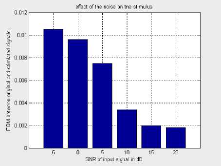
Fig. 11. Mean Quadratic Error vs SNR
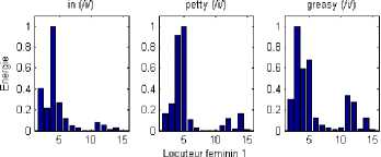
E. Energy Channel distribution
To confirm the last results, we have illustrated in the next fig.12 the sixteen channel energy coefficients computed from vowels and consonants localized in several words and pronounced by the same female speaker. We can observe a similar localization of the similar processed speech around 3 to 5 channels. For example, the most energy channels (which will be selected and excited) for the vowel /a/ in the words /dark/ and /had/ are the 4th,5th and 6th . This means that it is not necessary to stimulate all the channels but only the most 3 significant channels (cochlea electrodes) will be excited.
In fig.13 and fig.14, we can observe that the most significant channels are around the 13th, 14 th,15th and 16th channels contrarily to the vowels where the excited channels are between the 4th and the 8th channel. These results show a good correspondence between the vowels in different words and their positions. Besides, it enhances the discrimination between vowels and consonants and conduct to a better voice intelligibility.
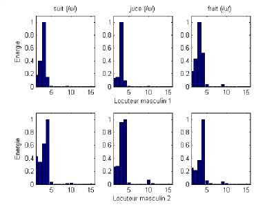
Fig. 12. Energy distribution of the three vowels /a/, /i/ and /u/ of the auditory channels in several words
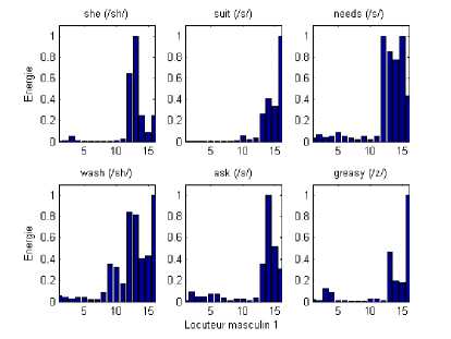
Fig. 13. Energy distribution of three unvoiced consonants /sh/, /s/ and /z/ of the auditory channels in several words (for a male speaker)
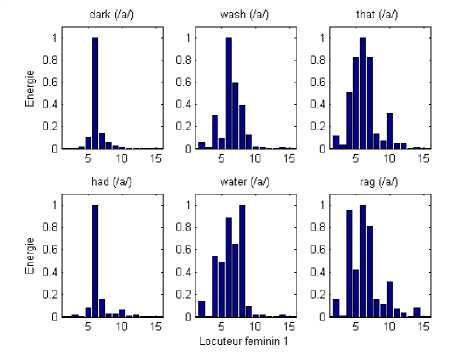
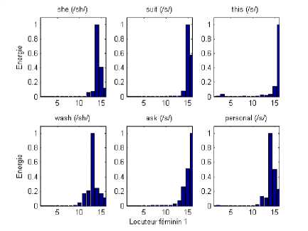
Fig. 14. Energy distribution of three unvoiced consonants /sh/, /s/ and /z/ of the auditory channels in several words (for a female speaker)
-
V. Conclusion
In this study, we presented a new auditory model based on the gammachirp filter-bank analysis. The parameters estimation of this model was conducted by comparison between the experimental Revcor strategy and the simulated auditory model responses. We succeeded to optimize the model parameters minimizing the mean quadratic error computed from the simulation results of the auditory model and the REVCOR experimental measurements. The implementation of this work was programmed with Matlab and C.
The simulation results have shown that a reduced number of 3 to 5 channels are sufficient to encode the speech signal. However, in noisy environments, it is necessary to compensate each SNR degradation of 5dB by adding three additional stimulation channels.
References Auditory Model Identification Using REVCOR Method
- M. Slaney Auditory, Auditory Toolbox, Technical Report 1998.
- M. J. Hewitt & R. Meddis: Implementation details of model computation of innerhair-cell for auditory-nerve synapse, journal of Acoustical Society of America, vol.87, no.4, p. 1813-1816, April 1990.
- M. Slaney: Lyons Cochlear Model, Apple Computer Technical report 13, 1988.
- S. Seneff: Mean-rate model of processing, journal speech auditory of Phonetics, pp.55-76, 1988.
- Carney, L.H., Megean j. Shkhter M, I.,“Frequency glides in the impulse responces of auditory-nerve fibers”, J.Acoust.soc.Am, No.4, pp.2384-2391, 1999.
- Boer, E.,and Nuttall, A. L. ‘‘The mechanical waveform of the basilar membrane. I. Frequency modulations in impulse responses and cross-correlation functions,'' Journal. Acoust. Am. 101, 3583–3592. 1997
- K. Ouni. Analysis of the vocal signal using of the acquaintances on the auditory perception and frequency time representation of signals. PHD Thesis ENIT, Tunisia 2003.
- H. Steven Colburn H. Laurel and Carney “Quantifying the implications of nonlinear cochlear tuning for auditory-filter estimates” JASA Journal, Vol 19. November 2001
- Earlab data viewer application, Hearing research center at Boston University 2009.
- T. Irino, D.Patterson. À time-domain, level dependent auditory filter : the gammachirp. J.Acoust of Am. 101(1): 12-419, January, 1997.
- M. H.Allerhand and Christian Giguere,"Time-domain modelling of peripheral auditory processing: À modular architecture and a software platform," Journal of the Acoustical Society of America, vol 98, pp 1890-1894, 1995.
- The Development System for Auditory Modeling http://www.essex.ac.uk/psychology/hearinglab/lutear/
- Patterson, R.D., Nimmo-Smith, I.,Wiber, D.L., and Milroy, R.,"The deterioration of hearing with age: Frequency selectivity, the critical ratio, the audiogram, and speech threshold", J.Acoust. Am., No.6, December 1982.
- Patterson, R.D., Nimmo-Smith, I.,"Off-frequency listening and auditory-filter asymmetry", J.Acoust. PloughshareAm., No.1, 1980.
- T. Irino, R.D. Patterson. Temporal asymmetry in the auditory system. J. Acoust. Am. 99(4):2316-2331, April, 1997.
