Automated Forecasting Approach Minimizing Prediction Errors of CPU Availability in Distributed Computing Systems

Published Online September 2016 in MECS

Many resources connected to the Internet are idle for most of the time. They represent a considerable reserve of computing power. Volunteer computing (VC) systems aim to harness this extensive number of underused computer resources and to reach a high computing performance. While these world-wide distributed resources are heterogeneous, unreliable and belong to independent administrative domains, appropriate middleware is deployed to aggregate, on-demand, the unused processing power. Tasks, submitted to a VC system by independent users, should be scheduled on the appropriate computing resources. However their availability, for VC system usage, is highly variable depending on demand, owners’ behavior, their time zones and their location (at home, school or work), etc. [1, 2, 38]. Consequently, the scheduler has no availability or speed guarantees. The scheduling optimization in such environments requires forecasting the future CPU resource availability.

A review of related works shows that there is no single prediction model which is optimal for all the considered CPU time series [3, 4, 5, 7]. Due to the diversity of world-wide distributed resources, the prediction accuracy is not always ensured using a single predictor. For such computing resources, the prediction system should be able to select automatically the appropriate predictor for each CPU resource among several integrated predictors. Besides, usual prediction systems are time consuming and consequently inappropriate for large-scale computing infrastructures [3, 8].

In this work, we are particularly interested in predicting CPU availability of volunteer resources in large-scale VC systems. For each computing resource, we predict precisely two CPU availability indicators (i.e. variables) that are the number and the mean duration of CPU availability intervals over the next hour. To reduce the solution time, we limit our study to simple approaches, which may outperform the most complex competitors [5, 9, 10] and ensure reasonable accuracies. We extend the approach proposed in [7, 9] in order to draw up guidelines to conceive a prediction system of resource availability in VC infrastructures. As pointed in [7], a volunteer resource may be in one of the three following states: totally available, totally unavailable or partially available over the whole hour. Multi-state based predictors are appropriate to forecast discrete values corresponding to the possible availability states of a resource. In this paper, we analyze the performance of several multi-state prediction techniques in order to retain the most accurate ones. We notice that their accuracies depend on the mean duration of the availability and unavailability intervals of volunteer resources. Consequently, we propose an automated approach to identify the appropriate multi-state prediction technique for each volunteer resource regarding its availability and unavailability frequencies.

For the totally available and unavailable states, the values of CPU availability indicators are known. However, in the case of the third availability state (partially available), the volunteer resource is unavailable during some intervals of the hour. So, CPU availability variables correspond to continuous value data. In order to predict their values, we require predictors such as time series models. Tendency-based strategy has been considered as an automated, simple and improved prediction technique referenced in many recent CPU load prediction researches [11, 4]. Autoregressive models have been shown to be among the simplest time series models using both autocorrelation and cross-correlation between multivariate time series [12, 7].They are as accurate as the most complex models [13, 5, 10]. Nevertheless, although they are well studied, their construction requires manual treatment [14]. Moreover, their successful usage requires the satisfaction of some assumptions in time series. To address these limits, we propose an automated method to construct the prediction models. We extend the utility of autoregressive models by exploiting three different past analyses. For a given resource, we analyze the CPU availability: first over the recent hours, second during the same hours of the previous days and third during the same weekly hours of the previous weeks. We extract subseries, corresponding to each past analysis, from the CPU availability time series. We check the main assumptions, such as correlation and stationarity in subseries, to be able to apply autoregressive models. We compare vector autoregressive (VAR) and pure autoregressive (AR) models, constructed according to our proposed approach, against the tendency prediction technique. We discard AR models from our study because they are the least accurate. We propose a heuristic which selects the appropriate predictor among VAR models analyzed over the three past analyses and the tendency based strategy.

The rest of this paper is organized as follows. Section 2 discusses related works. Section 3 reports a comparative study between tendency based strategy and autoregressive models constructed according to our proposed process and adapted to the three past analyzes. Section 4 presents the three-state availability modeling then describes and compares several multi-state predictors with respect to different subsets of volunteer resources. The proposed prediction system is presented in section 5 and evaluated in section 6. Finally, section 7 concludes the paper.

• II.    RELATED WORKS

Many characterization studies were conducted to predict the availability in VC systems. Besides, different prediction algorithms were used to predict resource availability and load in such large distributed systems. So, we organize this section accordingly.

A.    Parameter characterization to predict availability in VC systems

Early researches [15, 16, 17] were focused on characterizing host availability in VC systems. Some of them claimed that hosts in networks may be classified into two categories: those which are almost always online and those which have diurnal uptime patterns [16, 17].To predict host availability, some other characterization studies used parameterized models [40, 19]. Nurmi et al. [19] fitted statistical distributions to empirically uptime traces of machines. They derived some parameters from the models to estimate how long a random machine will remain available. Most of these researches focused on host availability which differs from CPU availability considered in this work. Host availability may be a deceiving metric as a host may be connected to the grid but its CPU may be unavailable to the grid usage because of user presence on the machine, local tasks execution, etc. However, we focus on CPU availability which is the time when the CPU of a host is available to run grid tasks as a volunteer resource.

In [1], as the goal was to characterize the correlated resources, authors did not consider the temporal dependence of resource availability. So, they represented each CPU trace by its average availability at each hour of the week. Then, they used k-means to classify resources into clusters with similar levels of availability. Besides, they exploited the clustering results to optimize the problem of resource selection and scheduling. In particular, to execute parallel applications, they selected the most rapid resources belonging to the cluster of highly available resources. Nevertheless, their approach did not consider the evolution of the availability behavior of volunteer resources during time. Indeed, due to its unreliability, a volunteer resource may belong to several clusters during different periods of time. Moreover, it was shown that the optimization of resource selection and scheduling problems, in such computing systems, relies on temporal structure of availability [20, 21]. Anderjeak et al. found that the average number of changes of the availability status per week is the most appropriate parameter to estimate the availability of a resource. They, regularly, computed availability parameters of resources and used them to forecast the amount of resources that will be available in the computing system [22].

These parameterized prediction methods based on characterization studies provide conservative estimates that facilitate dealing with the worst cases. However, they cannot be used to predict the evolution of the availability at multiple points in the future. Besides, they cannot accurately predict the availability of individual resources especially if the computing system is composed of heterogeneous hosts characterized by different availability behaviors.

Using randomness tests, Javadi et al. found that Seti@home resources had purely random [2] or autocorrelated [23] CPU availability and unavailability intervals. In [2], authors focused only on the 21% of the volunteer resources whose availability was random. They used clustering techniques to classify them into clusters of resources which can be modeled with similar probability distribution functions such as Gamma and hyper-exponential distributions. In [23], authors modeled the remaining 79% of volunteer resources whose availability and unavailability times were auto-correlated. They considered several other statistical models able to capture the long range dependency property that was discovered in time series. They found that, among the fitted models, Markovian Arrival Process (MAP) was the best. The fitting time of these models is relatively high because it depends on a high number of parameters. To adapt MAP models to large scale VC systems, authors reduced the number of these parameters by factors up to 50% and found reasonable accuracies. They claimed that, using some parameters derived from these statistical models, the scheduler could estimate the probability that a volunteer resource remains available or unavailable over a given future interval of time. However, this predicted probability does not depend on the prediction time. Moreover, models were fitted using all observations of the traces and were not tested on new unseen observations. To make use of these statistical models in our study, they have to be recomputed frequently in order to capture changes and dynamics in VC systems and enhance scheduling decisions. The resulting computing times may be relatively high, even reducing the number of parameters. Consequently, they are inappropriate to our case of study.

B.    Availability predictors

Many efforts have been made in host load prediction in grids and distributed computing systems using linear predictors [13, 10, 3, 24, 25] or non-linear predicators [5, 26, 27, 11]. All of them use combinations of the recent signal points to predict future points.

In [13], Dinda et al. found that the pure autoregressive AR(16) model outperformed the windowed mean (BM), moving average (MA) and LAST models when predicting host load. Besides, AR model had a lower computing time and a high precision, similar to ARMA, ARIMA and ARFIMA models. In order to improve CPU load prediction accuracy, Liang et al. proposed a multivariate AR prediction model, using both autocorrelation and cross-correlation between resources of a computing host [10]. The Network Weather Services (NWS) prediction system was proposed, including several prediction models such as: MEAN, LAST, BM, AR, MA, ARMA, etc. [3].Tendency prediction techniques were proposed to forecast the CPU load based on the polynomial fitting [24, 25] and information about previous similar patterns, i.e. successive decreases or increases between neighboring turning points [25]. According to the empirical studies, tendency prediction techniques outperformed AR(16) model and NWS.

In [4, 28], a CPU load prediction model was proposed based on the assumption that CPU load wave can be considered as the superposition of several small cyclic waves with different periods. First, the time series is decomposed into sub-sequences using Fourier transform [4] or wavelet packet decomposition [28]. At each prediction, tendency-based method [4] and revised ARIMA model [28] were used to predict the next value for each sub-sequence. Finally, the predicted values of all the sub-sequences were combined to deduce the final value. Experiments showed that, compared to the tendency-based predictor, this approach performed best for long-term prediction but worst for short-term prediction [4]. Compared to ARIMA model, this approach performed best for unstable time series which changes suddenly [28].

Although time series models are well studied, their successful application requires the satisfaction of some assumptions in time series. Besides, their construction requires manual treatment [14]. These limits reduce their utility for large scale dynamic computing environments. To address these constraints, some recent approaches checked assumptions in time series before applying time series models [5, 28]. To predict quality of service attributes such as response time, Amin et al. proposed an automated approach which selects among the linear ARIMA and the non-linear SETARMA models according to nonlinearity test [5]. All these predicators are appropriate for continuous value time series.

Using machine learning methods, for CPU availability prediction, promoted another category of related literature. To consider cross-correlation between resources of different grid hosts, Andrzejak et al. reduced the prediction problem to a classification problem by dividing the data range into a set of levels (classes) [26]. According to their comparative study between several classifiers such as Naive Bayes, k-Nearest Neighbor (k-NN) and decision trees, the Support Vector Machines (SVM) classifier was the most accurate [26]. Experiments showed that Support Vector Regression (SVR) outperformed NWS predictors [27]. In [8], a prediction system was proposed, including AR, Last and MA. A classifier, such as k-NN, was used to select the appropriate predictor. Historical data were pretreated using Principal Component Analysis in order to reduce data dimensions at the input of the classifier and consequently improve its performance. Results showed that such a prediction system outperformed NWS. In [11], a CPU load prediction strategy which combines Bayesian and Neuro-fuzzy inferences was proposed. This strategy outperformed AR, dynamic tendency proposed in [24] and NWS models. It performed as well as the tendency based technique proposed in [25].These non-linear predictors are appropriate for discrete value data. So, in order to use them, availability time series were discretized.

Compared to non-linear predictors, simple linear predictors, such as autoregressive time series models and tendency based strategy, have lower computing time and enough accuracy comparable to more complex competitors [5, 4, 11]. Similarly to pure autoregressive models (AR), Vector autoregressive models (VAR) were shown to be among the simplest prediction models considering both autocorrelation and cross-correlation between multivariate time series variables [12, 7].

To predict the availability behavior of resources at multiple points in the future, other predictors analyzed transitions between the availability states of each resource. Mickens et al. proposed a prediction system which selects the most appropriate predictor among several saturating counters and linear predictors according to an approach similar to that of NWS [29]. Saturating Counters (SC) predictors use the current state of a resource as the predicted value for the future time state. These simple predictors are attractive. This is because they use one bit to record state. However, they are not able to describe the availability over medium and long term time scales, unless using two or more bits to store the state. Other studies used multi-state-based predictors to predict the availability behavior of grid resources [30, 31, 32]. Statebased predictors use a multi-state model presented as a graph to denote transitions (edges) between states (nodes) in a recent availability history of a resource. Generally, the multi-state prediction algorithm takes as input an interval of time and a history of a resource. It produces as output a transition probability vector. Each element of the vector represents the predicted probability that the resource will transit to the corresponding state. Ren et al. proposed a multi-state prediction model including five states based on several levels of CPU load, memory thrashing and resource unavailability [30]. To predict the availability behavior during a given future time window, they counted transitions in the same time window on previous weekdays and weekends and used them to model a semi-Markovian process. According to their experiments, this multi-state predictor outperformed linear time series models. Rood et al. proposed another multi-state prediction model including five states; four of them were unavailability states due to user presence on the machine, excess of local load threshold, grid task eviction and host failures [31]. The fifth state is related to availability. Besides, they proposed and compared several prediction algorithms. According to their comparative study using Condor traces, “Transitional Day-of-week Equal weight” (TDE) and “Transitional Recent hours Freshness” (TRF) predictors were the best. The TDE predictor counts transitions during the interval being predicted on previous days. On the other hand, TRF predictor counts transitions over the recent hours favoring transitions that occur most recently. The TDE and TRF predictors outperformed Ren [30] and SC [29] predictors. In [32], Maleki et al. proposed a multi-state prediction model containing three states. They assumed that a CPU resource may be totally available, totally unavailable to the grid usage because of failures and membership cancelation or partially unavailable to the grid because its processing power is shared between grid and local tasks. Authors used continuous time Markov chains to predict the transition probability vector. These predictions were combined to performance metrics in order to improve scheduling decisions.

Due to the diversity of resources in VC systems, resources exhibit several availability patterns with different statistical properties such as auto-correlation, randomness, periodicity and steadiness [1, 2, 23].On the one hand, SC predictors perform well for resources which are most often available or unavailable [29]. On the other hand, multi-state based predictors perform well for resources which have periodic availability patterns [6].

Among these predictors TDE and TRF are the most accurate ones.

In this work, several predictors are integrated together in a unique automated prediction system, to improve accuracy. At each prediction, the most appropriate predictor is dynamically selected then used to predict the next value. Three automated selection methods of the best predictor were used in the literature: NWS method [3, 29], classification based method [8, 47] and the decision-rule based method [24, 25, 4, 5, 28]. First, using the NWS method, at each prediction, all the integrated models are run and the one with the least cumulative Mean Squared Error (MSE) is selected [3]. However, the cumulative MSE is an overall criterion which may be inappropriate to adapt the predictor selection to the changing CPU availability in VC systems. The second method aims at forecasting the best predictor then using it to predict the future value. A classifier, such as k-NN [8] and neural network [47], was used to select the best predictor. When many complex prediction algorithms are integrated, it is better to use the selection method based on classification instead of NWS, since only one predictor is run at any prediction step. However, both of these selection methods require the execution of all the prediction models either at each prediction step [3, 29] or at the construction of the classification model [8, 47]. So, both of them is time consuming and consequently inappropriate to large scale VC systems. The third selection method is less expensive as it selects the most appropriate predictor based on decision-rules. Nevertheless, it requires an expert knowledge to conceive the set of decision rules. To reduce computing time, our prediction system selects the appropriate predictor according to decision rules. Unlike most of the parameterized approaches, we need to predict the evolution of the availability of individual resources over time. To this end, the majority of the studies, described above, used their specific and limited availability traces not necessarily obtained from large scale volunteer systems [13, 24, 10, 25, 11]. Moreover, some of them focused only on hosts located in the enterprise or university [30, 31]. In contrast, as [2, 23], we consider real CPU availability traces of 226000 hosts [39] located in the enterprise, university and home. Unlike traces considered to evaluate the existing multistate availability models [30, 31], Seti@home traces do not report causes of unavailability. So, regarding the possible availability states of volunteer resources, we consider a multi-state availability model similar to that proposed in [32]. To predict the future availability state over the next hour, we use state-based predictors, such as: TDE, TRF and SC, due to their accuracy. If the resource is totally available or unavailable over the hour, values of the availability variables are known. Nevertheless, when the resource transits from one state to another, variables correspond to continuous value data. In this case, appropriate linear and non-linear predictors should be used. To reduce the solution time and improve the precision in a large-scale computing system, we consider simple predictors in the prediction system, in particular: autoregressive time series models and the tendency prediction technique. Moreover, we use vector autoregressive VAR to exploit the cross-correlation between the CPU availability indicators in order to improve the prediction accuracy. To address the limitations of the considered models, we check the main assumptions specific to the multivariate VAR and univariate AR models in time series. Moreover, as [5], we construct the prediction model according to an automated approach. Besides, we extend the utility of autoregressive models by exploiting different past analyses. Considering the repeated behavior of users, unlike [4, 28], we do not consider sophisticated decomposition methods. We, simply, limit our study to sub-series corresponding to daily and weekly hours. None of the considered predictors was evaluated using traces of large-scale VC systems. In this paper, we evaluate and analyze the performance of these predictors in order to retain the most efficient ones and acquire the knowledge required to conceive the prediction system.

• III.    LINEAR MODELS: ADAPTATION, PROPOSED CONSTRUCTION PROCESS AND EVALUATION

To reduce solution time and improve accuracy, we limit our study to linear predictors, in particular: VAR models, AR models and tendency prediction technique proposed in [25]. We focused on resources whose availability is auto-correlated due to repeated hourly, daily and weekly behavior of users. We also included resources that exhibit a combination of auto-correlated and random availability, for instance, those whose users’ behavior is similar every morning, unpredictable in the afternoons and almost the same at night. Consequently, the considered autoregressive time series models were adapted to different past analyses. Moreover, sub-series corresponding to the daily and weekly hours were extracted. To address the limitations of the considered time series models, the proposed automated approach checks assumptions in time series and constructs the prediction models by identifying their appropriate orders p without human intervention. We further extend the approach, described in [9, 7], to conceive a prediction system of resource availability in VC systems.

This section explains how VAR and AR models are adjusted to different past analyses. Their main assumptions are discussed and the proposed construction process of the prediction model is presented. Then, a comparative study, of the autoregressive models and the tendency prediction strategy, is reported.

A.    Adaptation of Autoregressive models to different past analyses

A vector autoregressive VAR(p, s) and pure autoregressive AR(p, s) models of order p, span s and lag (p*s) use the p past observations separated by s steps (hours) to predict the future values of the dependent variables. At each prediction, we considered three different past analyses as detailed in table 1 and consequently three VAR models and three AR models. For example, to examine the CPU availability during the same hours of the previous p days, we fixed the span s of the second VAR and AR models at 24 hour. In our study, for each past analysis corresponding to a given span s, we had exactly s sub-time series to extract from the original time series. Among them, we tried to identify the subtime series for which the assumptions of time series models were fulfilled i.e. for which the VAR and AR models could be constructed.

Table 1. Description of the three past analyses

Past Analyses	Description	Span s [hour]
1 st	Over the recent past hours	1
2 nd	During the same hours of the previous days	24
3 rd	During the same hours of the previous weeks	7*24

For example, according to fig. 1, to apply the second VAR and AR models ( s = 24), we tried to identify the ones among the 24 sub-time series which fulfilled the assumptions of time series models. So, a VAR model and an AR model were constructed for each hour of the day corresponding to predictable sub-time series. In total, at most 24 VAR models and 24 AR models may be constructed using the second past analyses. Although a sub-time series is a part extracted from a time series, in what follows, the two terms are used interchangeably.

B.    Assumptions of time series models

Each variable of the multivariate time series should, first, be auto-correlated over time. Second, it should be stationary: have constant mean (no trend), non-infinite constant variance over time and covariance function depending only on the delay between observations. Third, variables of the multivariate time series should be crosscorrelated, so that, the causality assumption is met i.e. each variable is helpful for predicting the other variable. Finally, time series models that are used to predict the future values should be stable i.e. errors should have finite values.

C.    The construction process of the prediction model

Fig. 1 illustrates our proposed approach to construct the prediction model. Before computing any time series model for a given past analysis of a resource, we check whether the time series meet the main assumptions of time series models using statistical tests. Otherwise, we try to find an appropriate transformation to fulfill these assumptions. In particular, we, first, check the autocorrelation using Ljung-Box test [33]. Secondly, if this condition is fulfilled, we check the stationarity using KPSS test [34]. If the time series are non-stationary, we transform them using the first difference and check the stationarity assumption for the differenced data.

After preparing the time series for each past analysis, we construct the VAR and AR models. To identify the most appropriate order of the model, we estimate several models for different values of p . All these estimated models are diagnosed in order to remove the inadequate ones and preselect the set of the fittest models. Among

Availability in Distributed Computing Systems the diagnoses, we, first, perform significance tests to retain models whose estimates (coefficient values) are statistically significant. For a given model, if all the estimates are statistically significant, they are kept in the model. Else, the model is recomputed using only significant estimates. Next, we perform Granger’s causality tests [35] to keep VAR models which agree with the cross-correlation assumption. Third, we carry out the portmanteau tests [33] to keep models whose error series are white noise process. Finally, we check the stability to retain stable models for which all the eigenvalues of the companion matrix are smaller than one in absolute value [12]. If this is the case, the stationarity hypothesis is fulfilled. Once the set of the fittest time series models is identified, we select the best VAR and AR models based on Bayesian information criterion (BIC) [36], particularly the one having the minimum BIC value.

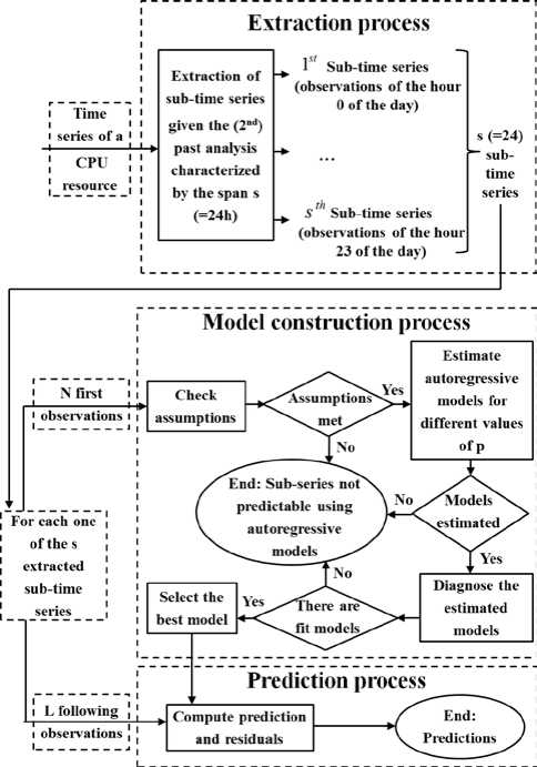
Fig.1. The proposed approach to construct the autoregressive model for a sub-time series

D.    Prediction

At each prediction time t , the future values of CPU availability indicators are predicted according to the three past analyses. For each past analysis, the best selected VAR (resp. AR) model, constructed using the sub-time series of the next hour t+ 1, is used to perform the prediction. Using the new observations, the prediction errors are computed.

E.    Evaluation

In this section, our evaluation study was conducted using CPU availability traces of 1000 hosts chosen randomly among 230000 hosts of Seti@home. These traces were recorded over the Internet, using the middleware BOINC [37], for more than 1.5 years between April 2007 and January 2009. Each trace reports the start and the end epoch times of CPU availability and unavailability events. The CPU availability is considered as a binary value indicating whether the CPU was free or not. So, traces of each resource were pretreated to deduce a multivariate time series which reports two variables that are: the number and the mean duration of CPU availability intervals per hour. In order to ensure enough samples to perform statistical tests for the three past analyses, we considered time series of a length longer than 50 weeks. We normalized them using the min-max normalization method. The prediction evaluation was performed in the walk-forward manner which consists in using a fitting interval of N observations to construct the models and an adjacent interval of L observations to perform predictions. Then, both intervals are moved forward by L and the process (of fitting followed by predictions) is repeated. We fixed N to 51 weeks and L to 1 week. To construct autoregressive models, we consider a maximum value of p equal to 24, 7 and 4 respectively for the first, second and third past analyses. At each prediction, the Absolute Percentage of Error (APE) was computed as the ratio of the absolute value of the prediction error (the difference between the predicted value and the real value) to the real value. The Mean Absolute Percentage of Error (MAPE) was computed as the average of the Absolute Percentages of Errors of all the predictions. All time series models and statistical tests were conducted using GRETL 1.9.12 [40] which is a C++ open-source library for which we were compelled to implement several necessary changes and additions.

Experiments showed that, in most cases, if the autocorrelation is met, then the stationarity is met, too. According to experiments, the number of CPU availability intervals is more predictable than the mean duration of CPU availability intervals. Limited by space, we report results for the least predictable variable. The main results reported below are well checked for the other variable.

According to fig. 2.a., AR models outperformed the other prediction techniques for less than 1% of the predictions. So, they should be discarded from our study. This may reduce the computing time of our prediction system. Fig. 2.a. also shows that tendency prediction technique outperforms VAR models for 82% of predictions. The majority of these predictions correspond to successive hours of availability or unavailability for which the predictor Last is used and the APE is equal to 0. VAR models outperform tendency prediction technique for only 18% of predictions. While this percentage is not large enough, the number of predictions, for which VAR models outperform tendency strategy, remains significant considering only intervals when the availability changes.

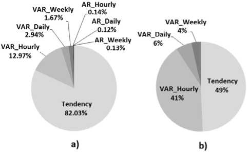
Fig.2. Percentages of predictions with respect to the best predictor: a) case of all predictions b) case of predictions performed when the availability changes

Fig. 2.b. shows the percentage of predictions, performed around intervals of availability variations, with respect to the best predictors. According to this figure, VAR models outperform tendency prediction technique for more than 51% of predictions performed when the availability changes. In particular, VAR models computed over the recent past, the daily hours and the weekly hours are the best predictors for 41%, 6% and 4% of these predictions, respectively.

Boxplots of APE of predictions, performed when the availability changes, are depicted in fig.3. Considering only intervals of CPU availability variations, VAR models produce a mean APE equal to 22.12% compared to 23.37% produced by tendency based strategy. So, using VAR models, when the CPU availability changes, improves the prediction accuracy by around 5.65%. Besides, the variation of the APE exhibited by VAR models for these predictions is significantly lower than that of the tendency based technique. Indeed, 50% of the APE are within [1.51, 24.76] so with a range equal to 23.25 for VAR models and within [0, 37.1] thus with a range equal to 37.1 for tendency based strategy. This indicates that the accuracy of predictions of VAR models is more stable across the different predictions than that of the tendency based technique.

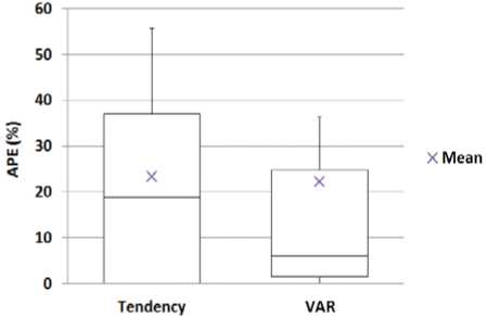
Fig.3. Box-plots of the APE of the predictions performed when the availability changes

F.    Retained lessons

We discarded AR models from our study because they are the least accurate. The predictor Last should be used if the availability remains constant. However, VAR models and tendency based strategy should be used when the availability changes because they are accurate enough. So, in order to select the appropriate predictor, the prediction system needs to predict, first, whether the availability will change. In other words, it requires estimating whether the availability behavior remains constant or not over the next hour.

• IV.    MULTI-STATE BASED PREDICTION

In order to select the most appropriate prediction technique to predict values of the CPU availability indicators, the prediction system requires forecasting whether the resource will transit to another availability state over the next hour. To this end, we retained statebased predictors due to their accuracy. In particular, we use TDE, TRF and SC predictors.

This section, first, introduces the proposed multi-state availability modeling and describes two proposed multistate predictors. Then, it presents a comparative study between these predictors and those retained from literature in order to identify the most appropriate ones for resources of VC systems.

A.    Availability modeling and multi-state predictors

We consider a multi-state availability modeling similar to that of [32]. However, we do not generate traces but, as mentioned above, we use real traces of Seti@home. From the perspective of the computing grid, the CPU of the volunteer resource may be in one of the three following states:

• •    Totally available, to the grid usage, over the whole hour: in this case, the entire processing power of the resource belongs to the grid environment during the whole hour.

• •    Unavailable, to the grid over the whole hour, due to failures, user present on the machine, turn off, etc.

• •    Partially available to the grid usage over the whole hour: in some intervals of the hour, the volunteer resource may be unavailable to the grid usage. In this case, only a part of its processing power is available to the grid usage during the hour.

The proposed modeling for the availability of a volunteer resource is shown in fig.4.

In addition, to improve the predictor TDE, we, first, propose to filter weekdays (working days) and weekends. TDEW denotes the predictor which operates as TDE but computes transitions over the same hours of the previous weekdays or weekends. Second, we propose to exploit the repetitive availability behavior over the weekly hours. TW denotes the predictor which counts transitions during the interval being predicted on the same days of the previous weeks. To further understand the differences between our proposed predictors and TDE, we present the following example. To predict the availability behavior at

11am on Tuesday using historical data of the previous four days, the TDE predictor counts transitions between 11am and 12am on Wednesday, Thursday, Monday and Sunday. However, the TDEW predictor computes transitions between 11am and 12am on Wednesday, Thursday, Monday of the same week and Friday of the previous week. On the other hand, the TW predictor performs the prediction based on the resource transitions exhibited between 11am and 12am, on each Tuesday of the previous four weeks.

Fig.4. The proposed multi-state availability modeling

We conducted several experiments to analyze the performance of the predictors. We noticed that the best multi-state predictor for a given resource depends on the frequency of its availability and unavailability events, i. e. whether it remains available or unavailable for most of the time or it changes frequently from an availability state to another. To this end, we tried to classify resources into groups according to the mean lengths of their availability and unavailability intervals. As detailed in table 2, we subdivided the range of the mean availability (resp. unavailability) intervals of resources into five orders of magnitude. In particular, for each resource, we consider that the mean availability (resp. unavailability) intervals may be in the order of minutes, hours, days, weeks or months.

In what follows, to identify the appropriate predictor, we conduct a comparative study between the five considered multi-state predictors that are: TRF, TDE, SC, TDEW and TW, with respect to the different groups of resources.

Table 2. Ranges of the mean availability (resp. unavailability) intervals

Order of magnitude	Length of the mean availability (resp. unavailability) interval [hour]
Minutes	Inferior or equal to 1
Hours	]1, 24]
Days	]24, 7*24]
Weeks	]7*24, 4*7*24]
Months	Superior to 4*7*24

B.    Evaluation

The evaluation of predictions was performed in the walk-forward manner using the 226000 traces of Seti@home hosts. We focused on traces which are longer than 50 weeks and for which host locations and time zones are mentioned. We define the multi-state predictor accuracy to predict the future availability states, for each resource, as the ratio of correct predictions to the total number of predictions. In this comparative study, the number of past hours, days and weeks was varied and the appropriate ones which maximize the prediction accuracy of the predictors were selected automatically for each resource. We considered a maximum value of 168 past hours, 60 past days, 60 past days and 48 past weeks respectively for the predictors TRF, TDE, TDEW and TW.

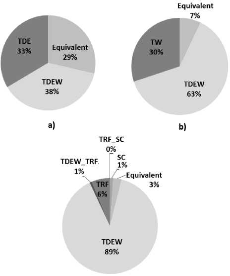
Experiments showed that, in average, the predictors TDEW, TDE and TW produce a mean accuracy equal to 94.34%, 94.29% and 94.24%, respectively. So, in average TDEW is slightly more accurate than TDE and TW predictors. According to fig.5.a and fig.5.b, the predictor TDEW is as accurate as TDE and TW for 29% and 7% of the considered resources, respectively. It is more accurate than TDE and TW for 38% and 63% of resources, respectively.

с)

Fig.5. Percentage of resources per best predictor: a) case of TDEW and TDE, b) case of TDEW and TW, c) case of TDEW, TRF and SC

According to fig.5.c, accuracies of TDEW, TRF and SC are equivalent for around 3% of resources. TDEW and TRF are equally the most accurate predictors for 1% of resources. TRF and SC predictors are the most accurate for 6% and 1% of resources, respectively. However, the predictor TDEW is the most accurate for 89% of the compared resources. Moreover, the mean accuracy of TDEW, TRF and SC are respectively around 94.53%, 92.47% and 91.56%. So, on average, TDEW outperforms TRF and SC predictors.

Figure 6 presents the percentage of resources per ranges of mean availability and unavailability intervals. Notice that the mean availability and unavailability intervals of the majority of resources are in the order of hours, days and minutes. A few resources are characterized by mean availability and unavailability intervals in the range of weeks and months.

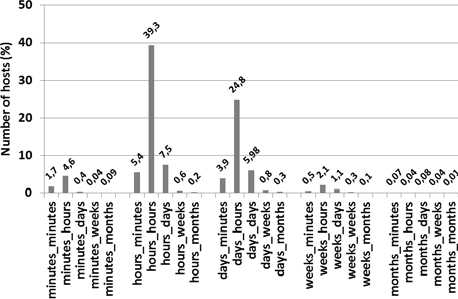
Availability „Unavailability

Fig.6. Percentage of resources per ranges of mean availability then unavailability intervals

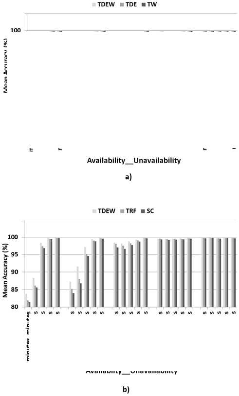
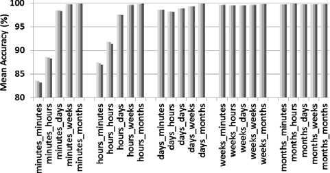
Fig.7. Accuracy of TDEW compared to other predictors: a) Case of TDEW compared to TDE and TW, b) Case of TDEW compared to TRF and SC

relatively variable. However, those corresponding to an order of weeks and months are more stable. Generally, it is more difficult to predict time series which are more variable than those which are relatively stable.

Figure 7.a presents the accuracy of the predictor TDEW compared to TDE and TW. For resources which have mean availability or unavailability intervals in the range of days, weeks or months, the predictors TDE, TDEW and TW perform similarly to one another. Their accuracy exceeds 97% for these resources which are mostly available or unavailable. However, for resources which have mean availability and unavailability intervals in the range of minutes or hours, TDEW is slightly more accurate than TDE and TW predictors. For these subsets of resources whose time series are highly variable, the accuracies of the predictors are about 83% to 92%.

According to figures 7.b. and 8, TDEW is the most accurate for the majority of resources which have mean availability and unavailability intervals up to the range of days. Its accuracy increases with the range of the availability and unavailability intervals, from 83.64% up to 98.88%. For this first subset of resources, TDEW reaches an accuracy increase of up to 4% over TRF and up to 5.25% over SC. So, TDEW is appropriate to predict the availability states of this first subset of resources. On the other hand, TRF becomes slightly more accurate or similar to TDEW for resources which have mean availability (resp. unavailability) intervals in the range of weeks or months (resp. months). Nevertheless, the difference in accuracy is small and all the compared predictors have a high accuracy exceeding 99%. It is worth-reminding that the number of this second subset of resources is quite small. Time series are relatively stable as CPUs remain available or unavailable for most of their time. Consequently, using TFR to exploit the recent past may be more useful and less expensive to predict the availability states of this second subset of resources.

«Equivalent TDEW = TDEW_TRF -TRF TRF_SC ■ SC

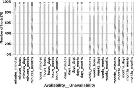
Fig.8. Percentage of resources per best prediction algorithm among TDEW, TRF and SC

As we can see in figure 7, the predictor accuracy increases with the length of the mean availability and unavailability intervals. This may be explained by the fact that, time series of resources whose mean availability and unavailability intervals are of order up to days are

• V.    PREDICTION SYSTEM MODELING

The proposed prediction system selects the most appropriate predictor using a multi-state prediction technique. Then, it uses the selected predictor to predict the CPU availability indicators.

In this section, we, first, introduce the proposed prediction algorithm which uses VAR models or tendency strategy based on decision rules. Then, we describe the proposed approach to identify the appropriate multi-state prediction technique for each volunteer resource. Finally, we present the prediction system.

A.    The prediction algorithm using linear predictors

Experiments showed that VAR models outperform tendency prediction technique for a significant number (around 51%) of predictions performed when the availability changes. In particular, VAR models computed over the daily and weekly hours are the best predictors for around 10% of these predictions. Moreover, the three subsets of resources, for which VAR models are computed over the different past analyses, are complementary rather than overlapping. Consequently, when the availability is expected to change, we propose to predict CPU availability indicators using a prediction heuristic which identifies the most appropriate predictor according to decision rules. This heuristic integrates VAR models over the three past analyses and tendency based technique. To this end, we evaluated different conceivable prediction heuristics with several reversed combinations of the three past analyses. Experiments showed that the different resulting prediction systems have similar prediction errors.

In what follows, we retain the prediction heuristic denoted RDW which selects the appropriate predictor according to decision rules favoring the recent, the Daily then the Weekly past analyses and finally the tendency based strategy (fig.9.). At the prediction time t, assumptions of time series models are checked. Once the autocorrelation and stationarity assumptions are met for a given past analysis, then the corresponding VAR model, constructed using the sub-time series of the next hour t+1, is used to perform the prediction. If none of the VAR models computed over the three past analyses is selected, then the tendency based strategy is used to carry out the prediction. Using the new observations, the prediction errors are computed.

At the prediction time t,

• 1.   if models’ assumptions are met for the previous hours, then

• 2.   if models’ assumptions are met for the same hours of the

• 3.   if models’ assumptions are met for the same weekly hours of

• 4.    use the tendency based strategy.

use VAR Hourly . Else,

previous days, then use VAR Daily . Else

the previous weeks, then use VAR Weekly . Else,

Fig.9. The proposed heuristic RDW

B.    The approach to identify the most appropriate multistate prediction technique

As shown in section IV.B, the magnitude of the mean availability and unavailability durations are useful to identify the appropriate multi-state prediction technique for each volunteer resource.

For the small subset of resources which have a mean availability (resp. unavailability) interval in the range of weeks or months (resp. months), TDEW is a little less accurate than TRF and relatively similar to TDE, TW and SC predictors. For these volunteer resources, exploiting the recent past seems more appropriate to predict the availability behavior which is relatively stable. Consequently, we propose to use TRF predictor for this subset of resources.

For the other resources whose time series are relatively variable, errors are so high. The predictor TDEW is both significantly more accurate than TRF and SC and slightly better than TDE and TW. So, TDEW is the most accurate predictor and consequently the most appropriate one for these resources.

Fig. 10 presents the proposed approach to identify the appropriate multi-state prediction technique for a volunteer resource in order to predict its future availability state.

For a given volunteer resource,

• 1.   if the mean unavailability interval is in the range of months,

• 2.   if the mean availability interval is in the range of weeks or

• 3.   if the mean availability interval is in the range of minutes,

then use TRF. Else,

months, then use TRF. Else,

hours or days, then use TDEW.

Fig.10. The proposed approach to identify the most appropriate multistate predictor for a volunteer resource

C.    The prediction system

Now, we combine both techniques, described above, in the prediction system. Before performing predictions, at each walk-forward step:

• •    the mean availability and unavailability durations are computed;

• •    their ranges are identified according to table 2;

• •    the appropriate multi-state prediction technique is identified according to the approach proposed in fig.10;

• •    and VAR models are constructed according to the process described in fig.1.

At each prediction time t, giving historical data of the volunteer resource, the multi-state prediction technique is used to estimate the probabilities of transitioning to another state from the current state and the probability to remain in the same current state during the next hour. The future state of the volunteer resource is predicted according to these probabilities. In particular, it corresponds to the highest probability. If the CPU is predicted to be partially available to the grid usage over the next hour then the heuristic RDW is used to predict the availability indicators. Otherwise, if the volunteer resource is predicted to remain in the same availability or unavailability state, then the predictor Last is used to perform the prediction. If the volunteer resource is predicted to be available (respectively unavailable) over the whole next hour, then the mean duration of the availability intervals is estimated to be equal to 1 hour (respectively 0). The proposed prediction system denoted PS is shown in fig.11.

• VI.    EXPERIMENTS AND EVALUATION

The prediction evaluation was performed in the walkforward manner. We considered the same experimental setups described in section 3.5. Moreover, for each volunteer resource, we used 168 past hours and 20 past days to perform pred ictions according to TRF and TDEW, respectively. At each walk forward step, we used historical data of the three past months to identify ranges of the mean availability and unavailability durations. Experiments were run on a linux based laptop equipped with an Intel 2.20 GHz dual core i7 processor inside and a 4 GB memory.

At each prediction time t,

• 1.    Use the multi-state prediction technique to forecast the future availability state.

• 2.   if the volunteer resource is partially available then use

• 3.   if it remains in the same availability or unavailability state,

• 4.    if it is available, then both availability indicators will be

• 5.   if it is unavailable, then both availability indicators will be

RDW. Else,

then use LAST. Else,

equal to 1. Else,

equal to 0.

Fig.11. The proposed prediction system PS to predict the availability indicators of a volunteer resource

A.    Applicability of the prediction system

We evaluated the PS using 226000 CPU availability traces of Seti@home hosts. Among them, we ignored 47% of hosts for which the location and the time zone are not indicated. In order to ensure enough samples to perform statistical tests for the three past analyses, we considered traces longer than 50 weeks. About 80% of hosts do not have enough samples. Finally, we applied the PS to 22424 traces (about 20% of the considered hosts). Although the number of considered hosts is not large enough, they remain significant considering their deliverable computing power gathered over the large-scale computing system. In total, their time series correspond to 4687 years of CPU time. The considered hosts are well distributed throughout the time zones and locations as those considered in [1, 2]. In particular, 77% of them are located at home, 20% at work and 3% at school.

B.    Accuracy of the muti-state predictor

In this section we evaluate the ability of the PS to predict the future availability states of the resources. Worth-reminding that, at each walk forward step, PS identified the appropriate predictor among TDEW and TRF according to the approach presented in fig.10.

Experiments showed that TDEW predictor was used to perform the majority (around 91%) of the predictions.

However, TRF predictor was used for only 9% of the predictions. This may be explained by the fact that few subseries are relatively stable. For the prediction of these subseries, PS used the TRF predictor. This fact is confirmed in fig.6 which shows that the majority of time series are not stable but quite variable.

The mean accuracy of PS to predict the availability states is high (around 94.05%). Fig.12 presents the accuracy of the multi-state predictors used by PS for the different subsets of predictions. The mean accuracy of the TDEW and TRF predictors are around 93.31% and 98.91% respectively.

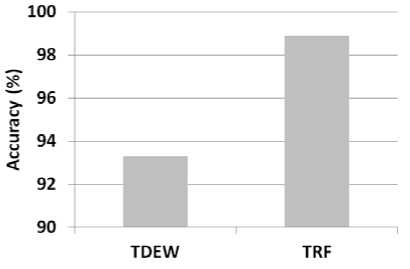
Fig.12. Accuracy of the multi-state predictors used by PS

C.    Accuracy of the prediction system

In this section, we compare the proposed PS to the predictor Last in order to predict the availability indicators of the resources. The mean MAPE of the PS is equal to 2.43%. The PS is slightly better than Last whose mean MAPE is around 2.77%. At first, we believed that this slight difference may be because the PS used the predictor Last for many times. Experiments, however, showed that this is not the case. The PS used Last for only 4.36% of the predictions. However, our PS and Last are similar for 90.42% of the predictions. Hereafter, we ignored predictions for which errors of the PS and LAST are similar. We limited our evaluation to the 5.22% remaining predictions for which APEs of the PS and Last are different. Although the number of these predictions is limited, they correspond to more than 244 years of CPU time. Experiments showed that the majority (more than 97%) of these predictions were performed when the availability changes. In particular, they correspond to hosts whose time series are relatively variable.

Fig.13. presents the box-plots of MAPE of hosts. It indicates that, when the PS and Last are equivalent, MAPE of resources are very low with a mean equal to 0.98%. Moreover, 50% of the MAPE of hosts are within [0.18%, 1.44%] so with a range equal to 1.26. However, when errors are different, the PS produced a mean MAPE equal to 16.54% compared to 20.5% produced by Last. So, using our prediction system improves the prediction quality by around 24%. Besides, the variation of the MAPE, exhibited by the PS for these hosts, is significantly lower than Last. Indeed, 50% of the MAPE of hosts are within [8.42%, 23.03%] so with a range equal to 14.61 for the PS and within [11.69%, 29.82%] thus with a range equal to 18.13 for Last. This indicates that the accuracy of the PS is more stable across the different hosts than that of LAST.

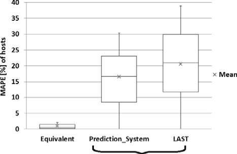
Not Equivalent

Fig.13. Box-plots of MAPE of hosts computed when the errors of our prediction system and Last are equivalents and different

• VII. CONCLUSION

In this paper, we propose an automated approach to identify, at each prediction time, the most appropriate prediction model, for a given volunteer resource, according to the nature of its time series. To this end, we analyzed the performance of several prediction techniques. We extended the usefulness of autoregressive models analyzed over the recent past by exploiting two other different past analyses. Our approach was evaluated using real CPU traces of the large scale computing project Seti@home. The comparative study showed that VAR models outperform the other considered prediction techniques for a significant fraction of predictions. We retained the most suitable models in order to reduce solution time and to minimize prediction errors. Considering their accuracy, VAR models combined to the tendency-based strategy should be used when the availability changes. To predict whether the resource availability will change, the adequate multi-state prediction technique is identified, then, used. Accordingly, the most appropriate prediction model is selected among the retained models. On average, the proposed approach improves the accuracy by around 24%.