Automatic brain tissues segmentation based on self initializing K-Means clustering technique

Published Online November 2017 in MECS

Image segmentation is an important image processing technique that partitions the image into number of homogeneous regions based on the characteristics of the pixels [1]. Segmentation depends on various features like regions, edges, color, and texture etc. of the image. Thus the segmentation techniques are categorized into threshold based, edge based and region based segmentation. Threshold based image segmentation allocates the pixels into categories according to the range of pixel values. Edge based image segmentation groups the pixels into edge or non- edge depending on the edge filter’s output, applied to the image. Region based image segmentation algorithms operate pixels iteratively by grouping neighbors with similar values [2].

Segmentation and clustering techniques can be applied in various fields in the medical domain to analyze and identify the abnormalities present in organs like human heart, bone of knee and brain [3] [4]. The abnormalities form in brain due to any of the disorders like tumors, seizure, stroke, trauma and head injury etc. The diagnostic process based on manual segmentation by medical experts is time consuming. Hence Computer Aided Diagnostics (CAD) systems are aimed in medical field at present [5].

There are various modalities available for imaging organs, some of which are computed tomography (CT), magnetic resonance imaging (MRI), electroencephalography (EEG), magneto encephalography (MEG) and positron emission tomography (PET). MRI uses radio waves in a strong magnetic field to create detailed images of organs and tissues. MRI has been proven to be highly effective in diagnosing normal and diseased tissues of the body and produces more accurate results [6].

The MR images provide a large amount of data with high quality when compared with other modalities data. It provides good contrast between the soft tissues of body. Thus the segmentation in MRI results better classification of brain tissues, its surrounding fluid and background. The classification of these tissues will help to analyze and study the anatomy and functions of brain [7]. Algorithms are derived to segment different types of tissues in organs like gray matter (GM), white matter (WM), cerebrospinal fluid (CSF) and tumor region (if it is an abnormal brain) in MRI brain image [8].

K-Means clustering is one of the hard segmentation algorithms used in various applications. But the main limitation of this algorithm is the selection of number of clusters and initial centroids to segment the given input data. In digital image processing, the selection of initial centroids can be done automatically using many ways.

The proposed method uses image histogram to get the initial centroids and the number of clusters automatically and named as Histogram Based Self Initializing K-Means (HBSIKM) method. Experiments were done with the MRI brain volumes available from Internet Brain Segmentation Repository (IBSR). Similarity validation was done by Dice coefficient with the available gold standards from the IBSR website. The performance of the proposed method is compared with the traditional K-Means method. The similarity results show that the proposed method runs efficiently in segmenting the tissue regions with minimum number of iterations and also with the self-initialized centroids of MRI brain images. For the IBSR volumes, the proposed method yields 3 to 4 times faster results and higher dice value than traditional K-Means method.

In this paper, section II contains the related works done and section III contains the methodology. The results are discussed in section IV and conclusion is given in section V.

• II.    Related Work

Kaufman and Rousseeuw have proposed an algorithm to initialize the K-Means segmentation by manually selecting the K-value [9] [10]. The first centroid is selected as the most centrally located instance and the other centroids are taken as the higher numbered instances among the rest of data in the database. The limitation is the manual initialization of the number of clusters and their centroids. Bapusaheb and Bansode have developed Pillar algorithm in which the first centroid is taken as the grand mean of the dataset [11]. The data point with a maximum distance from the previous centroid is taken as the next centroid. Thus the other centroids are found out in an iterative manner by calculating the distance metrics. But it has the limitation of adjusting the characteristics of data distribution in dataset, in order to set up the appropriate parameters for outlier detection mechanism.

Tian et al., have proposed a method to automatically initialize the K-Means clustering algorithm based on histogram of the input dataset [12]. In this algorithm, all the local maxima in the histogram are taken and the global maxima among them are selected as the first centroid. And the remaining centroids are taken iteratively with the help of a maximized distance measure (DM). The DM is the product of height of local maxima and the distance from previous centroids. Here the limitation is manual selection of centroids and K (no. of classes) value. Mohamed et al., have proposed an EI-Kmeans algorithm that made improvement over the K-Means segmentation algorithm by introducing a novel density function based on k-nearest neighbor method [13]. By this definition the noise and other outliers that affect Kmeans strongly are obtained along with the initial centroids and number of clusters automatically.

Raed has done the initialization of centroids based on calculating the Euclidean distance and Manhattan distance between the data points and centroids [14]. But this process starts with randomization of the centroids. Kalaiselvi and Somasundaram have proposed an algorithm called FCM-Expert where the initialization to four clusters is done manually from the knowledge of the MRI brain scan images [5]. Here the peak values from the histogram are taken in to consideration. The background intensity is taken as 0 and white matter as 255 and the peak values 85 and 170 are taken as centroids to cerebrospinal liquid and gray matter respectively. The fixed values initialization is done with knowledge based technique.

In the proposed method, the initialization is done automatically with the help of histogram of the gray scale MRI brain image. The middle slice in an MRI volume is considered to have all the tissue regions thus its histogram is chosen to get the initial K and their centroid values. The number of peaks and their values are taken to initialize the number of classes and the centroids in the K-Means algorithm. The final centroids of each slice are used to initialize the adjacent slice’s K-Means segmentation process. The pre-processes involved in the proposed method are brain portion extraction and bounding box cropping to remove the unwanted background from the input image. Finally, the performance evaluation is done by comparing the results with the ground truth values available from IBSR datasets.

• III.    Methodology

K-Means segmentation is an unsupervised classification algorithm that needs the manual initialization of the number of classes as well as randomization of initial centroids of each class. The initial cluster is created by associating each pixel in the image to the given nearest centroid, then the mean values of the elements in the clusters are computed and the centroids are replaced by them. These steps are done iteratively until there is no more in centroid [15]. The traditional K-Means algorithm is given below.

Algorithm 1: K-Means clustering

Step 1 : Set K and C, the number of clusters required and initial centroids randomly.

Step 2 : Allocate each pixel to the nearest class. This is done by minimizing the objective function J as given below.

J =∑f=l ^∑7=1 || X ^{( 1} - Cj ||²             (1)

where, ‖ X ⁽⁷ - ^ci ‖ is a chosen distance measure between a data point x ⁽⁷⁾ and the cluster center ^ci . It is an indicator of the distance of the n data points from their respective cluster centers.

Step 3 : Compute mean value for each cluster and replace the new centroid as the mean value.

Step 4 : Repeat steps 2 and 3 until no more new centroids are created.

The main aim of the Histogram Based Self Initializing K-Means (HBSIKM) method is to fully automate the K-Means clustering algorithm using the normalized histogram of the MRI gray scale. Fig. 1 shows the flow chart of proposed method. The three main processes of the proposed method are brain portion extraction, bounding box cropping and histogram based centroids initialization. Brain portion extraction is done by BEM algorithm for each image. As a result the brain region alone is extracted [6]. The bounding box technique is applied on this image to ignore unwanted background and crop the AOI that is the brain portion alone. Then the histogram is taken for the middle slice of each dataset since the middle slice is considered to have all the tissue regions clearly. This is done in order to get the exact number of clusters and their centroids in the MRI brain dataset. Gaussian smoothening is applied over the histogram to get distinct peaks. The automatic initialization of the number of clusters (K) is done with the number of peaks and initial centroids with the peak values of the normalized histogram. With these initial K and C values, the K-Means segmentation is performed on each slice in the dataset. For each time the final centroid of the current slice is taken as the initial centroid for the next slice in the dataset. These three processes support to enhance the performance of traditional K-Means method by reducing the number of iterations in the segmentation of each image and thus the time too.

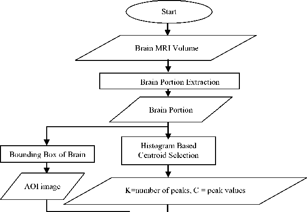
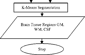
Fig.1. Flow chart of the proposed method

Algorithm 2: HBSIKM

Input : MRI volume

Step 1 : Apply BEM algorithm to extract brain portion.

Step 2: The image histogram of the middle slice generated.

Step 3: Apply Gaussian filtering on the histogram in order to smoothen the histogram that yields distinct peaks. The Gaussian distribution is

1    - ⁽ -μ)

^G( X ) = a √2 /- ₂²              (2)

Step 4: Find the number of peaks K and peak values C .

Step 5: Initiate the number of clusters K by m and the initial centroids Cj by a where j=1, 2…K. for the middle slice in the dataset.

Step 6: Select the AOI using bounding box cropping process.

Step 7: Apply K-Means segmentation for the AOI.

Step 8: Use the final centroids of the previous slice to initialize the centroids for current slice

Step 9: Repeat the previous two steps for the remaining slices in the dataset.

• A.    Brain Portion Extraction

The MRI brain image contains three portions skull, scalp and the soft brain inside. Here the AOI is the brain portion where the three main tissues GM, WM and CSF reside. Thus the first step is to extract the region of interest i.e. the brain portion from the skull and scalp. For this the BEM is applied. This is a fully automatic two-stage brain extraction method that extracts the brain portion from the MRI images using feature extraction in first stage and morphological and connected component operations in the second stage to produce the fine brain portion. A sample coronal MRI image is shown in Fig.2 (a) and its extracted brain portion is given in Fig.2 (b). This sample image corresponds to the middle slice of 205_3 voulme from IBSR20 dataset.

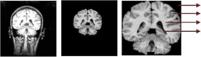
Background Gray Matter White Matter CSF

Fig.2. a) Sample MRI head scan b) Extracted brain after BEM c) AOI after bounding box cropping

(a)

(b)

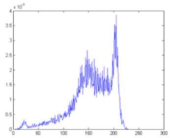
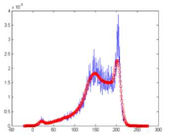
Fig.3. (a) Histogram (b) smoothed histogram

• B.    Bounding Box Cropping

The bounding box technique is applied on the resultant image of the previous step in order to extract the brain portion alone as the AOI by cropping the unwanted background. This is done in following steps.

Algorithm 3: Bounding Box Cropping

Step 1: Scan the input image row wise from top to bottom until a row with a data >0 is reached. This row is taken as rowmin .

Step 2: Scan the image row wise from bottom to top until a row with a data >0 is reached. This row is taken as rowmax .

Step 3: Scan column wise from left to right until a column with data >0 is reached. This column is taken as colmin.

Step 4: Scan column wise from right to left until a column with data >0 is reached. This column is taken as the colmax .

This bounding box algorithm is applicable for MRI brain images since the background is set to zero by BEM. The AOI of the image lies within the rowmin, colmin and rowmax, colmax coordinates of the image. The cropped AOI image with the indication of BG, CSF, GM and WM is shown in Fig.2(c).

• C.    Histogram Based Centroid Selection

Image histogram is the graphical representation of the intensity distribution over the pixels of the image. The histogram of the middle slice is taken in order to get the number of tissue regions present in the brain image and also contains the most frequent intensity value in each region. Since the middle slice is considered to have all the tissue regions, it is selected for the histogram based centroid selection. The low pass Gaussian smoothening filter is applied on the histogram as given in equation (2) in order to get the distinct peaks. The histogram produces peaks corresponding to the number of regions present in the brain image. Since the brain has three main regions CSF, GM and WM, the histogram produces three main peaks that is taken as the number of centroids K, and the corresponding peak values for Cj (centroid of each region) where j=1, 2, 3….K. The histogram and the smoothened histogram with distinct peaks for the middle slice of IBSR 205_3 dataset are shown in Fig.3 (a) and Fig.3 (b) respectively.

• D.    K-Means segmentation

K-Means segmentation in the proposed method begins with the initial K as the number of smoothened peaks and the centroids Cj as the peak values in the histogram, taken for the AOI portion of the middle slice. Because of the adjacency nature among the slices of the MRI volume, the final centroids of each slice is taken as the initial centroids for the adjacent images. The K-Means clustering is performed as given in Algorithm 1.

• E.    Evaluation Metrics

The Dice coefficient is an index to measure the similarity of the segmentation. It is calculated as

2 | A ∩ В |

| A | + | В |

where, A and B are the pixel count of the respective regions in ground truth image and segmented image. The performance evaluation of the proposed method is done by calculating Dice coefficient (D) and compared with that of traditional K-means clustering algorithm.

• IV.    Results and Discussions

The experiments were carried out on 20 and 18 – Coronal T1 weighted IBSR datasets. Initially each slice is applied with the brain portion extraction algorithm in which the segmentation of brain portion is done in two stages. The first stage performs feature extraction where a rough brain portion is extracted with the help of run length identification for labeling the brain, scalp and background, skull and CSF. In the second stage a fine brain mask is created using morphological and largest connected component operations. In this stage, the adjacent slice’s similarity property is used to select the proper brain regions. As a result the brain portions are extracted for each slice in the above said datasets.

The proposed HBSIKM and the traditional K-Means algorithms are applied on the resultant images of the BEM algorithm. From each dataset, the slices with the major brain portions were taken for the processes by leaving the end slices present in both ends of the dataset in order to avoid the wastage of time, since these slices contains less amount of brain information.

The histogram of the input brain portion is taken for the middle slice of the dataset, and Gaussian smoothening is applied on the histogram in order to get distinct peaks. From the smoothened histogram the number of centroids and the initial centroids are taken for further processing. Then the bounding box cropping is done on all the slices in order to avoid the unwanted background. With these initial values the K-means segmentation is performed on the all the slices from the beginning of the dataset except those slices with less brain portions by carrying the final centroids of one slice to the next slice’s initial centroids.

As the result of above said segmentation processes, the three main tissues CSF, GM and WM of each slice are obtained. The respective sample images are shown in Fig. 4. Figure 4 contains the smoothened histogram with distinct peaks in column1, the original image, the CSF region, the GM region, the WM region and the triclustered region images in column 2, 3, 4, 5 and 6 respectively. The CSF region contains the sulcul CSF around the GM in the result of proposed method.

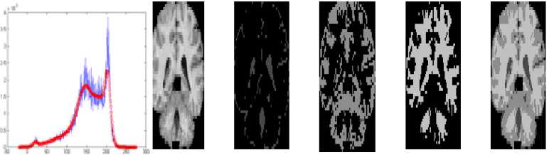
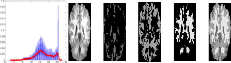
Fig.4. Results of proposed HBSIKM method Column 1: Smoothened histogram, Column 2: Original slices, Column 3: CSF region, Column 4: GM region, Column 5: WM region and Column 6: tri-clustered image.

Traditional method

(a)

Traditional method

Average no. of Iterations

я

я

я

(b)

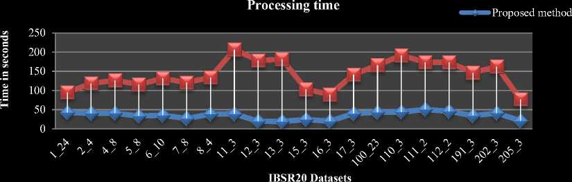
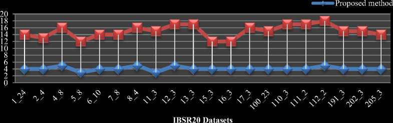
Fig.5. Performance comparison of traditional and proposed methods on IBSR20 volumes a) Processing time comparison b) Average iteration count comparison

In the proposed method, since the initialization is done automatically and the centroids are carried over to the adjacent slices to initialize their centroids, the number of iterations and the time taken to segment for each slice is reduced. The comparisons between the traditional as well as the proposed methods are shown in Fig 5, 6, 7 and 8.

The comparison between the traditional as well as the proposed algorithms in terms of average time taken and the number of iterations to segment per slice of each volume in IBSR20 datasets are shown in Fig.5 (a) and Fig.5 (b) respectively.

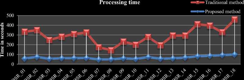
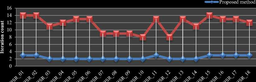
The comparison chart for average time taken per volume in IBSR18 is shown in Fig.6 (a). The comparison chart for average iteration count per slice of each volume in IBSR18 dataset is shown in Fig.6 (b). From Fig.5 and 6 our proposed HBSIKM algorithm is approximately 3 to 4 times faster than the traditional K-Means algorithm. A quantitative analysis is performed to examine the segmentation by calculating the Dice coefficient between the ground truth and the resultant images of traditional and proposed methods.

IBSR18 Datasets

(a)

Average no. of Iterations

Traditional method

IBSR18 Datasets

(b)

Fig.6. Performance comparison of traditional and proposed methods on IBSR18 volumes a) Processing time comparison

• b) Iteration count comparison

Table 1 shows the comparison between the average Dice coefficients of the results of HBSIKM and traditional K-Means for IBSR20 datasets. The final mean dice value of IBSR20 datasets is shown in Fig.7 as bar chart. Since the gold standard for these volumes consist SCSF, the similarity coefficients for CSF have increased.

Table 2 shows the comparison between the average Dice coefficients of the results of proposed and traditional K-means for IBSR18 dataset. The final mean dice value of IBSR 18 dataset is shown in Fig.8 as bar chart. Since the proposed method’s CSF region includes the Sulcal Cerebrospinal Fluid (SCSF) in the surrounding, and it is not included in the corresponding IBSR gold standard images, the similarity coefficients for the corresponding segmentation results have got reduced for IBSR 18 dataset.

Table 1. Average Dice coefficient of each volume in IBSR20 dataset

Volume	Traditional K-Means			Proposed HBSIKM
	CSF	GM	WM	CSF	GM	WM
1_24	0.1538	0.7086	0.8424	0.1463	0.7368	0.8466
2_4	0.1385	0.6456	0.7559	0.0683	0.5929	0.7421
4_8	0.1148	0.6644	0.7366	0.1888	0.6500	0.7704
5_8	0.0667	0.6677	0.7845	0.1964	0.7235	0.8266
6_10	0.0584	0.6710	0.7577	0.2657	0.7022	0.8219
7_8	0.0667	0.7198	0.8355	0.1416	0.7336	0.8483
8_4	0.1270	0.7160	0.8156	0.1693	0.7306	0.8368
11_3	0.0333	0.7209	0.8335	0.2444	0.7565	0.8683
12_3	0.0635	0.7158	0.8425	0.2595	0.7650	0.8868
13_3	0.0952	0.7114	0.8447	0.0763	0.7190	0.8687
15_3	0.0833	0.5955	0.6506	0.2203	0.6226	0.7107
16_3	0.1500	0.6828	0.7477	0.1596	0.6790	0.7762
17_3	0.1111	0.6912	0.8076	0.1738	0.6790	0.8337
100_23	0.1587	0.7259	0.8303	0.1043	0.7490	0.8729
110_3	0.1270	0.7477	0.8229	0.1681	0.7572	0.8457
111_2	0.5542	0.1094	0.7004	0.1546	0.7561	0.8597
112_2	0.1270	0.7419	0.8222	0.1546	0.7385	0.8246
191_3	0.1111	0.7373	0.8437	0.1260	0.7531	0.8580
202_3	0.0952	0.7300	0.8438	0.2604	0.7722	0.8698
Mean	0.1282	0.6686	0.7957	0.1725	0.7167	0.8299

Mean Dice for IBSR20

• • Traditional method

• ■ Proposed method

  

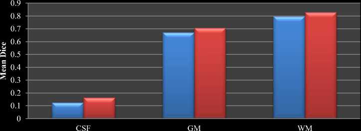
  Fig.7. Mean Dice comparison between traditional and proposed HBSIKM for IBSR20 dataset

  
  

Table 2. Average Dice coefficient of each volume in IBSR18 dataset

Volume	Traditional K-Means			Proposed HBSIKM
	CSF	GM	WM	CSF	GM	WM
IBSR_01	0.5294	0.7572	0.7966	0.5177	0.7755	0.8194
IBSR_02	0.6600	0.8175	0.8578	0.6464	0.8106	0.8448
IBSR_03	0.6350	0.7957	0.7750	0.6056	0.7927	0.7779
IBSR_04	0.5213	0.7926	0.7805	0.4570	0.7968	0.8370
IBSR_05	0.7094	0.8048	0.8269	0.7034	0.8160	0.8466
IBSR_06	0.7579	0.7057	0.7703	0.7469	0.7375	0.8077
IBSR_07	0.5634	0.7693	0.8750	0.5295	0.7655	0.9002
IBSR_08	0.6361	0.7651	0.8650	0.6140	0.7675	0.8866
IBSR_09	0.5585	0.7637	0.8873	0.5368	0.7550	0.8937
IBSR_10	0.6230	0.7812	0.8874	0.6026	0.7765	0.8995
IBSR_11	0.5286	0.7481	0.8720	0.5188	0.7477	0.8801
IBSR_12	0.5951	0.7635	0.8465	0.5796	0.7717	0.8738
IBSR_13	0.5530	0.7952	0.7822	0.5099	0.7998	0.8209
IBSR_14	0.6839	0.8501	0.8492	0.6540	0.8521	0.8656
IBSR_15	0.4869	0.8008	0.8466	0.4693	0.8020	0.8614
IBSR_16	0.4932	0.8068	0.8372	0.4603	0.7948	0.8410
IBSR_17	0.4949	0.8051	0.8314	0.4755	0.8165	0.8581
IBSR_18	0.4992	0.8036	0.8516	0.4598	0.7899	0.8705
Mean	0.58492	0.7848	0.8355	0.5604	0.7871	0.8547

• ▼ Traditional method

Mean Dice for IBSR18

• ■ Proposed method

  

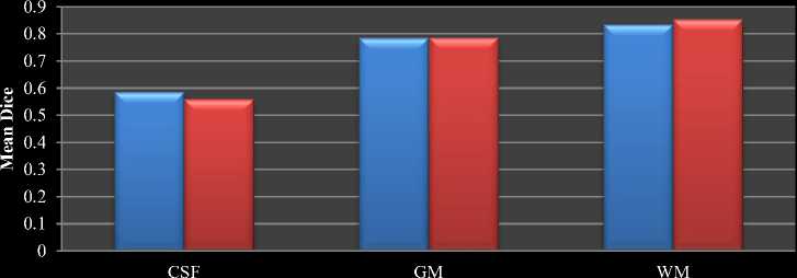
  Fig.8. Mean Dice comparison between traditional and proposed HBSIKM for IBSR18 dataset

  
  
  

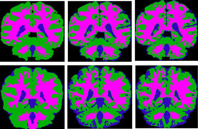
  Fig.9. Segmented portions of CSF in blue color, GM in green color, WM in pink color. Column 1: Ground truth image, Column 2: Results of the traditional method and Column 3: Results of the proposed HBSIKM method

  
  

The colored combination of CSF,GM and WM of ground truth, traditional K-Means results and proposed HBSIKM method results are shown in Fig. 9 in columnwise respectively for the qualitative level comparision.

The proposed HBSIKM method shows better results than the traditional K-Means segmentation. Further our proposed method is faster than the traditional method. If the data volume is affected by any artifacts then the initialization process by the middle slice yields wrong results sometimes. This is considered to be a limitation of the proposed work. In future, a preprocessing related to artifact removal will be considered to prevent this overhead.

V. Conclusion

In this paper a histogram based self-initializing K-Means segmentation algorithm (HBSIKM) has been proposed that initializes the K-Means technique automatically by the knowledge of MRI images and histogram processes. The experiments were carried out on 20 and 18 T1 coronal IBSR datasets. The results show that the proposed method speeds up the processing by reducing the number of iterations for each slice. Further the similarity measures of the proposed method shows better results than the traditional K-Means method