Balanced Quantum-Inspired Evolutionary Algorithm for Multiple Knapsack Problem

Published Online October 2014 in MECS

0-1 Multiple Knapsack Problem (MKP) is a generalization of the standard 0-1 knapsack problem (KP) where multiple knapsacks are considered to be filled instead of one. The MKP problem is strongly NP-complete and no FPTAS is possible for MKP [1].

Evolutionary Algorithms (EAs) refer to a class of population based search technique used to obtain good solutions for hard optimization problems in general. Individuals in population map to solutions of the problem. The new generations are evolved with an objective to improve quality of solutions. Evolution of a new population involves application of various operators on members of existing population. Quantum-Inspired Evolutionary Algorithms (QIEAs) is subclass of EAs where the representation of individuals and operators involved in generation of new individuals are both designed based on the concept of Quantum Computing.

Various forms of QIEAs have been used to solve a variety of difficult problems for example [2,3,4,5,6,7,8,9, 10,11]. QIEAs have been observed as a powerful tool because of their better representation power [12,13], EDA style of functioning [14,15], flexibility necessary for the inclusion of features appropriate for a given problem towards delivering better search performance [15], inherent quality of starting with exploration and gradually shifting towards the exploitation [13].

QIEA in itself only provides a very broad framework. QIEA, just as other EAs, suffers from several limitations. Small qubit rotations lead to slow convergence while large qubit rotations may cause the algorithm to miss a good solution completely. Inclusion of features promoting faster convergence may cause the algorithm to get stuck in local optima. Slow convergence limits the problem sizes that can be tackled using QIEAs. Implementation of QIEAs, therefore, is more an art. Any attempt to solve a difficult problem has to use this framework judiciously and include features suited to the particular problem in order to get the desired performance. The objective in any attempted implementation of QIEA is to balance exploration and exploitation thus achieving convergence to optimal or near optimal solutions without requiring prohibitively large computation even for larger problem sizes.

Hybridizing the population based meta-heuristic search technique with heuristics algorithms available for particular problem is an approach that is popular since last few decades to solve difficult optimization problems [16]. The main motivation behind the hybridization of different algorithms is to exploit the complementary character of different optimization strategies. Hybrid meta-heuristic algorithms try to establish a balance between exploration and exploitation of the search space.

The population based search approaches are good at exploration of the search space and identifying areas with high quality solutions while they are not so effective in exploitation of these high quality areas. On the other hand the strength of local search is the capability of quickly finding better solutions in the vicinity of starting solutions. Generally the heuristics available for optimization problems are based on some kind of local search on an initial solution. Thus in such algorithms, which hybridize a meta-heuristic with a heuristic, the meta-heuristic approach can guide the global search and problem domain specific heuristic can help searching locally around the good solutions found from global perspective.

Modifications	reference e.g.	Type	Maximum Size n= items count m= knapsacks count
Original QIEA (QIEA-o)	[17,18]	KP	n=500
Modified initialization of Qubit individuals in QIEA	[18] [19] [20] [21]	KP KP KP KP	n=500 n=500 n=500 n=500
Modification in Termination Criteria	[18]	KP	n=500
Modification in attractor, gate, etc while Updating the qubit	[18] [4] [3] [11] [22]	KP KP DKP QKP MoK	n=500 n=500 n=10,000 n=200 n=750,m=4
Modifying Repair function based on domain knowledge	[19]	KP	n=500
Replacing local and/or global migration of QIEA-o with other strategy	[23] [24]	KP KP	n=500 n=500
Incorporation of genetic operator mutation	[3] [11]	DKP QKP	n=10,000 n=200
Changing number or length of q bit individuals	[25]	MoK	n=750,m=4
Reinitialization of Qubits	[23]	KP	n=500
Inclusion of domain knowledge in the search process.	[26] [25] [3]	MoK MoK DKP	n=750, m=2 n=750, m=4 n=10,000
QIEA-o with parallel implementation	[27]	KP	n=500
QIEA-o implementation on GPU	[28]	KP	n=250

*KP= 0/1 Knapsack Problem, MoK = Multi-objective Knapsack Problem, QKP = Quadratic Knapsack Problem, DKP= Difficult 0/1 Knapsack problems

In this paper an attempt is made to design a hybrid QIEA balanced in its power to exploit and explore the search space in order to solve instances of MKP. The population based meta-heuristic QIEA is hybridised with an existing heuristic for MKP known as MTHM [29] and some additional features of population based search are judiciously incorporated in order to solve randomly generated instances of MKP. This is first attempt to solve MKP using such a meta-heuristic technique.

The rest of the paper is organized as follows. A brief description of MKP with a survey of approaches existing in literature for MKP is presented in section II. A brief conceptual description of a typical QIEA is given in section III. The MTHM heuristic used for hybridizing QIEA is discussed in section IV. In section V the QIEA framework used here and the proposed QIEA-MKP is explained in detail. Computational performance of QIEA-MKP is presented in section VI. Conclusions are presented in section VII.

• II.    MULTIPLE KNAPSACK PROBLEM (MKP)

Given a set of n items with their profits p j and weights W j , j E ^{1,.,n^} , and m knapsacks with capacities c i, i E ^{1,..., m^}, the MKP is to select a subset of items to fill given m knapsacks such that the total profit is maximized and sum of weights in each knapsack i doesn’t exceed the capacity c i .

maximize : ^m=i sp=i PjX(1)

subject to :XJn=1wJx1J < ci, iE{1,^,m},(2)

1т=1Хц< 1, jE{1,^,n},(3)

x1jE{0,1}, V1E{1,...,m], VjE{1,...,n], where xij = 1 if item j is assigned to knapsack i, xij = 0 otherwise and coefficients pj, wj and ci are positive integers.

In order to avoid any trivial case, the following assumptions are made

• 1.    Every item has a chance to be placed at least in largest knapsack:

• 2.    The smallest knapsack can be filled at least by the smallest item:

• 3.    There is no knapsack which can be filled with all items of N:

maxjENwj< maxiEU^.m} ci.

^^{1,..^} ci< minjENwj.

Zjn=1Wj> ci, ViE{1,..., m!.(7)

The subset sum variant of MKP having

Pj = w j ,jE^{1,^,n}, is known as multiple subset sum problem (MSSP).

MKP has many applications in fields related to computer science and operations research. An application is seen when scheduling jobs on processors where some machines unavailable for a fixed duration or some high propriety jobs are pre-assigned to processors [30]. A real world application of MKP is the problem of cargo loading where some containers need to be chosen from a set of n containers to be loaded in m vessels with different loading capacities for the shipment of the containers [31]. Another real world problem for MSSP is mentioned in [32] from a company producing objects of marble. The company receives m marble slabs, of uniform size, from a quarry. Each product, that company produces, requires a piece from marble slab having a specified length. Out of the list of products to be prepared, some products need to be selected and cut from the slabs so that the total amount of wasted marble is minimized. This problem is modelled as MSSP with slabs corresponding to knapsacks and the lengths corresponding to the weights.

Several attempts to solve the MKP exist e.g. [33,29,34] etc. Hung & Fisk [33] presented a depth first branch and bound algorithm where the upper bounds were derived by Lagrangian relaxation. Martello & Toth [29] proposed a different branch and bound algorithm where constraint S™ i X ij < 1 is omitted at each decision node and the branching item was chosen as an item which had been packed in k>1 knapsacks of the relaxed problem. In a later work Martello & Toth [34] proposed a bound and bound algorithm where at each node of the branching tree both the upper bound and lower bound are derived.

represents a superposition of 2n binary states and provides an extremely compact representation of entire space.

The process of generating binary strings from the qubit string, Q, is known as observation. To observe the qubit string Q, a string consisting of the same number of random numbers between 0 and 1 (R) is generated. The element P i is set to 0 if R i is less than square of Q i and 1 otherwise. In each of the iterations, several solution strings are generated from Q by observation as given above and their fitness values are computed. The solution with best fitness is identified. The updating process moves the elements of Q towards the best solution slightly such that there is a higher probability of generation of solution strings, which are similar to best solution, in subsequent iterations. A quantum gate is utilised for this purpose [17].

Procedure QIEA-original

• 1      t ← 0

• 2       initialize Q(t)

• 3      make P(t) by observing the states of Q(t)

• 4       repair P(t)

• 5       evaluate P(t)

• 6       store the best solutions among P(t) into B(t)

• 7     while ( t

• 8        {

• 9        t ← t+1

• 10        make P(t) by observing the states of Q(t-1)

• 11         repair P(t)

• 12         evaluate P(t)

• 13        update Q(t)

• 14         store the best solutions among B(t-1) and P(t) into

B(t)

• 15         if (migration-period)

• 16           {migrate b or b l to B(t) globally or locally,

respectively.}

• 17       }

Fig. 1. Quantum Inspired Evolutionary Algorithm

One such gate, used by the QIEAs presented in this work, is the Rotation Gate, which updates the qubits as follows:

^] - [

cos(Δθi) sin(Δθi)

-sin(Δθi) cos(Δθi)

ilя

I II . Q UANTUM I NSPIRED E VOLUTIONARY A LGORITHM (QIEA)

The QIEAs introduced in [17] are population-based stochastic evolutionary algorithms. They use the qubit, a vector, to represent the probabilistic state of individual. Each qubit is represented as q_;- J^¹], а₁,в₁ are complex numbers so that |a i I² is the probability of state being 1 and |в, I is the probability of state being 0 such that la i ^|2+|в,| =1 . For the purpose of QIEAs, a and в₁ are assumed to be real. Thus, a qubit string with n bits

where, α_i^t+1 and β^t+1denote probabilities for i^th qubit in (t + 1)^th iteration and Д0 , is equivalent to the step size in typical iterative algorithms in the sense that it defines the rate of movement towards the currently perceived optimum.

The above description outlines the basic elements of QIEA. Observing a qubit string ‘n’ times yields ‘n’ different solutions because of the probabilities involved. The fitness of these is computed and the qubit string Q is updated towards higher probability of producing strings similar to the one with highest fitness. This sequence of steps continues; these ideas can be easily generalised to work with multiple qubit strings.

• IV.    M THM H EURISTIC FOR MKP

• 1.    Initial feasible solution is obtained in the first phase of MTHM by applying the Greedy algorithm to the first knapsack; a set of remaining items is obtained, then the same procedure is applied for the second knapsack; this is continued till the m^th knapsack.

• 2.    The initial solution is improved during the second phase by swapping every pairs of items assigned to different knapsacks and insert a new item such that the total profit is increased.

• 3.    Each selected item is tried to be replaced by one or more remaining items during the last if possible so that the total profit sum is increased.

The MTHM heuristic has the advantage that some items can be exchanged from a knapsack to another or excluded from the solution set so that total profit increases, which can lead to an efficient and fast solution when the solution given by the first phase is good. Moreover they can be applied to any feasible solution effectively. The main drawback of MTHM heuristic is that it considers only the exchanges between a pairs of items and not the combinations of items.

Various phases of this heuristic can be introduced in QIEA to improve the quality of solutions found. In section V use of these to improve the performance of QIEA-MKP is examined in detail. The first phase of this heuristic is used to repair the infeasible solutions generated by collapse operation of QIEA. The second and third phases are applied as local search technique on the solutions improved from global perspective during the iterations of QIEA.

• V.    QIEA-MKP

The above description provides a broad framework of QIEA with scope for enhancements for rapid solution of a specific problem. This frame work is used as the starting point here which has been enhanced with several features. The modified algorithm designed for MKP is named as QIEA-MKP. The improvements brought about in QIEA-MKP are as follows.

(i)The items are sorted in order of decreasing profit by weight ratio to improve the domain knowledge in the following

• a.    Initializing the Qubit Individuals so that they generate better solutions.

• b.    Modifying the repair function to improve quality of solutions.

• (ii)    Improving the local best solutions using local search

• (iii)    Mutation of solutions when they appear to be stuck in a local optimum

• (iv)    Re-initialization of Qubit individuals (v) Local exploitation before global exploration

• A.    Sorting of items in input

The items having a greater profit by weight ratio are considered to have higher probability of their inclusion in the optimal solution. Thus the items in input are sorted in the decreasing order of their profit by weight ratio. This sorting is used to initialize qubit individuals so that they can generate better solutions and also to improve repair procedure so that it provides better solutions.

Initializing the Qubit Individuals to depict the better estimations of distribution models: In order to initialize the qubit individuals, the items are divided in to 3 classes based on where they lie in order of preference; the first class contains items having high preference for selection in a knapsack, items in second part have intermediate preference and third contain items having low preference. Hence, qubits for items lying in first class (third class) are assigned values closer to 1 (0) so that they have high (low) probability of collapsing to value 1. Items lying in the second class require more processing for convergence to either 0 or 1, hence intermediate values between 0 and 1 are assigned to them.

As a result, QIEA-MKP starts exploiting the area or region in solution space having higher probability of having solutions closer to optimal.

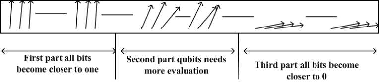
Fig. 2. Initialization of qubits. Qubits for items shown are sorted in decreasing profit by weight ratio from left to right

Procedure RepairMKP (x)

• 1    let R ←с ^-∑r=i ԝjxij, ∀ і ∈ {1,…,m};

• 2     for i from 1 to m{

• 3        while (R < 0) {

• 4         u ← max _∀ j ∈ { ,…, } (ј)|xij =1

• 5       x ←0; R = R +w ;

• 6        }//*while*//

• 7      }//* for i*//

• 8        for j from 1 to n {

if (k =   mіn ∀ ∈ { ,…, } (і)|R ≥ wi   )

{x kj ←1; Rк=Rк-ԝj;}

• 10       } //*for j*//

Fig. 3. Pseudo-code for RepairMKP

Modifying the repair function to improve quality of solutions: QIEA uses a simple “repair” function after it observes the qubits through the “make” procedure to make the observed solution feasible. In QIEA-MKP, the repair function is modified to improve the quality of solutions while making them feasible based on the phase 1 of MTHM heuristic presented in section IV. This improves the speed of convergence. As explained earlier the items are sorted in order of their preference to include them into a knapsack. So, in each repair step, items closest to the end are removed and items closest to the beginning are added as necessary. The knapsacks are assumed to be sorted in order of their increasing capacity and that’s the order in which they are considered when items are added into knapsacks. The pseudo-code is given in Fig. 3.

• B.    Improving the local best solutions

The local best solutions are further improved in two stages based on the phases 1 and 2 of MTHM heuristic [29] described in section IV. In first stage it tries to exchange every pair of items assigned to different knapsacks along with inserting a new item so that total profit is increased. Secondly, every selected item (starting from last in the sorted order) is tried to be replaced by one of the remaining items so that the total profit sum is increased. The pseudo-code of these procedures is given in Fig. 4. and Fig. 5.

• C.    Mutation of solutions appearing to be stuck in local optimum.

EAs suffer from tendency of getting stuck in local optima. All the modifications described above help the algorithm to exploit the search space around the greedy solutions increasing the speed of convergence but they also increase the tendency to get stuck in local optima. To combat this problem, if a new solution generated is seen to be close to global best solution found so far it is mutated. During mutation, after 2-3 bits in the solution vector are randomly selected and changed to 0, the partial solution is improved using ImroveStage1. To check closeness of two solutions, Hamming distance between them is calculated. Such an operator improves diversity without increasing the computational effort. It helps to explore the solution space around a current solution such that local optimal in vicinity is not missed. This improves the chances of finding optimal in case it is in vicinity of the converging solution.

Procedure ImproveStage1(x)

• 1    let R ←с -^∑P=i ԝjxij, ∀ і ∈ {1,…,m};

• 2    for each pair i and j in {1,…,n}{

• 3     if ( ∃ u,v іn {1,… ,m}| x =1 and xVj =1 and (R ≥

ԝj-ԝ) and (R ≥ w - wj)){

• 4       if ( ∃ k ∈ {1,…,n} | (R ≥ w j +w_k-ԝ ) or (R ≥

ԝ+ wк- wj)){

• 5            let k = ( mіn_∀ s ∈ { ,…, } s   | (R ≥ wi+w -

• ԝ) or (R ≥ԝ + w - wj))

• 6          if  ( (R ≥ wj+w -ԝ ){ x  ←0; xVj ←

0;xU) ←1; x ←1;xuk←1;}

• 7          else { x ←0; xvi ←0;xui ←1; x ←1;xvk ←

1;}

• 8          }//* if*//

• 9        }//* if*//

• 10   }//*for pair i and j*//

Fig. 4. Pseudo-code for ImproveStage1

Procedure ImproveStage2(x)

• 1    let R ←с -^∑P=i ԝjxij, ∀ і ∈ {1,…,m};

• 2    for ∀ і ∈ {1,…,n}{

• 3      if ( ∃ u ∈ {1,…,m}|x  =1){

• 4       for ∀ ј ∈ {1,…, n}|xVi =0 ∀ v ∈ {1,…,m} {

• 5           if(R_u + w_i - w j ≥ 0) P j ← p -p ; else P j ← 0;

• 6          }//* for j*/

• 7          let P k =max ∀ j ∈ { 1 ,…, n } P j ;

• 8         if( P k >  0 )  { x ui ← 0; x uk ← 1;R u ← R u + w i -

• wk ;}

• 9        }//*If u *//

• 10    }//*for i *//

Fig. 5. Pseudo-code for ImproveStage2

• D.    Re-initialization of Qubit individuals.

It may happen even after applying mutation as explained in section 5.3 that all the solutions generated from a qubit individual are still same after a sequence of generations. It clearly indicates that such a qubit individual has converged and no further new solutions can be generated using them. Thus, each qubit in individuals which generate same solution for more that 3 times out of 5 is reset as explained in section 5.1. It increases the diversity of solutions explored through the qubit individuals without increasing the computational effort.

• E.    Local exploitation before global exploration.

QIEA has the property that it updates the qubits over the time period such that they represent Estimation of Distribution models. Thus, basic steps of QIEA are executed for some iterations to update some of the qubit individuals initialized as described in section V.A.1. The steps listed in the following are performed on half of the qubit individuals for small number of times (empirically set as 15 for this work) before starting QIEA-MKP on the entire population.

• •    Make

• •    RepairMKP

• •    ImproveStage1

• •    ImproveStage2

• •    Update

The execution of these steps of QIEA will also exploit intensively the area represented by the current qubit individuals before starting the QIEA-MKP which is balanced with respect to its power of exploitation and exploration. The resulting qubit individuals thus favour the small solution subspace close to better solutions.

A solution to MKP must specify whether the item is included or not and if it is included then the index of knapsack it has been put into. Hence an optimal solution does not require only the selection of correct items but also that they are packed into the correct knapsacks. In this work, two components (in the form of two binary strings) are used to represent a solution individual where, first of length n contains 0 or 1 for each item conveying about its selection status, and second of length (n*log2 m) contains the index in binary of knapsack in which it is packed. The integers in {1, …, m} are represented by a bit string of length log2 m. A qubit individual is thus represented by two components of lengths n and n*log2 m correspondingly.

The complete pseudo-code for QIEA-MKP is presented in Fig. 6. In the pseudo-code for MKP; t refers to the current iteration, two components of population of qubit individuals after t^th iteration are represented using Q1(t) and Q2(t), P1(t) and P2(t) represent the population of individual solutions, B1(t) and B2(t) is the set of best solutions corresponding to each individual, c i is the capacity of the i^th knapsack. Individuals represented by Q1(t) and Q2(t) are referred to as q^t (composed of q1^t and q2^t), individuals in P1(t) and P2(t) are referred to as p^t (composed of p1^t and p2^t), similarly individuals in B1(t) and B2(t) are referred to as b_j^t (composed of b1_j^t and b2_j^t) for each j ∈ n ; b refers to global best solution having components viz., b1 and b2. In the following paragraph a brief description is given for procedures called in QIEA-MKP but have not been described yet.

InitializeGreedy (q1^t): where q1^t is j^th qubit individual in a population Q1(t). The procedure initializes the qubit individual q^t as explained in section V.A.

Make P1(t) and P2(t) from Q1(t) and Q2(t): The procedure collapses the qubit individuals in Q1(t) (or Q2(t)) observing solution individuals in P1(t) (or P2(t)).

HamDistance ( p1^s , b1): Returns hamming distance between two binary strings.

Mutate ( p1^s): Mutates the solution p1^s as described in section V.D.

Update q^t based on b_j^t: Rotates the qubits q1^t towards bits in b2_j^t and q2^t towards bits in b1_j^t as explained earlier and defined in [17] using the rotation angle as 0.01.

Evaluate P(s) : Assign individuals in P(s) to their profit values.

The maximum number of iterations in algorithm is controlled using a global constant, MaxIterations.

• VI. R ESULTS AND D ISCUSSION

  The experiments are done on Intel® Xeon® Processor E5645 ( 12M Cache, 2.40 GHz, 5.86 GT/s Intel® QPI ). The machine uses Red Hat Linux Enterprise 6.

The solutions converged for most of the problem instances considered here within 10 iterations hence maxIterations is set to 10. Empirically, η t and η 2 are set to 5 and population size is set to 10.

The experiments are performed to observe the effect of the modifications presented in sections V.A through V.E on basic QIEA framework discussed in the beginning of section V. The performance of QIEA and QIEA-MKP is observed on randomly generated instances having elements 1000, 5000 and 10000 with number of knapsacks as 2, 5 and 10.

The problem instances are randomly generated, using the generator of instances available at the Pisinger’s home page viz. , where weights wj are distributed in [1, R] and profits pj are calculated as pj = wj + R/10. Such instances correspond to a real-life situation where the return is proportional to the investment plus some fixed charge for each project.

Two different classes of capacities are considered for the knapsacks in randomly generated instances viz., similar and dissimilar. In instances with similar capacities the first m-1 capacities ci , i□{1,…,m-1} are distributed in

[0.4 ∑jn=1 wj⁄m ,0.6 ∑jn=1 wj⁄m] □i□{1,…,m-1} while instances with dissimilar capacities have these ci distributed in

• *0,0.5 (∑_jⁿ₌₁ w_j - ∑ⁱ_k^-₌¹₁ c_k)+ for i=1,…,m-1         (10)

The last capacity cm in both classes is chosen as

• c_m = 0.5∑_jⁿ₁w_j -∑_i^m₁¹c_i                  (11)

Tables 2 and 3 present the performance of QIEA and QIEA-MKP for the instances having similar capacities. Tables 4 and 5 present the performance of QIEA and QIEA-MKP for the instances having dissimilar capacities. Instances are randomly generated with number of elements ranging from 1000 to 10000 and number of knapsacks ranging from 2 to 100. The instances having 100 knapsacks of dissimilar capacities could not be generated.

Procedure QIEA-MKP

• 1    SortGreedy the Input;

• 2    t ← 0; b ← 0;

• 3    InitializeGreedy ( q1*) for eachj E[1,., n};

• 4     Initialize q2 * to 1 /V 2 for each j E [1,., n * log₂m};

• 5    Make P1(t) and P2(t) from Q1(t) and Q2(t);

• 6    RepairMKP (P1(t));

• 7    copy P1(t) to B1(t) and P2(t) to B2(t);

• 8    for each j E[1,., n/4} {

• 9       Make p* from q*;

• 10     RepairMKP (P1(t));

• 11      ImproveStage1 (P1(t));

• 12      ImproveStage2 (P1(t));

• 13      if ( p * is better thanb j ) b * < p *

• 14   }

• 15    while ( t

• 16     t ^ t+1;cnt j ^ 0 ;

• 17     for r from 0 to η do

• 18       for s from 0 to η do

• 19           Make P(s) from Q(t);

• 20          RepairMKP (P(s));

• 21            Evaluate P(s);

• 22             for each j E[1,.,n} if ( p^s better than p * ) p *

^ p s ; else cn* j ^ cn* j + 1;

• 23         } //*for s*//

• 24       for each j E[1,., n} {

• 25            if      ( HamDistance (      p^s     ,b)<2)

{ Mutate ( p^s); ImproveStage1 ( pj);}

• 26         }//*for j*//

• 27       if(cn(> 3 ){

• 28             InitializeGreedy ( q1*) for each j E [1,., n};

• 29             Initialize q2 * to 1 /V 2 for eachj E[1,.,n*

log m};

• 30         }//*if cnt j *//

• 31         for j E [1,..., n/2} ImproveStage2 ( p*);

• 32         for each j E [1,.,n} if ( p * is better than b j )

• 33        for each j E [1,., n} if (b j is be**er*han b) b^ b j ;

• 34        for each j E [1,., n} Update q* based on b * ;

• 35      } //*for r*//

• 36     for each j E[1,., n} Update q* based on b;

• 37   } // *while*//

Fig. 6. Pseudo-code for QIEA-MKP

The tables show a comparison of profit values obtained using the specific format of QIEA with values obtained using the heuristic mentioned in section IV. The best, average, worst, standard deviation in profit values obtained within 30 independent runs of the algorithm have been reported along with the minimum and average computaional effort required in terms of number of function evaluations (FES) as to reach the best (MinFES and AvgFES respectively) and RDH relative distance of best solution from heuristic. If profit for the instances obtained using exact algorithm is P h and best profit obtained is P b the RDH is calculated as follows.

RDH= (fa -Ph )/Ph ) *100                (12)

The convergence of profit values achieved using QIEA and QIEA-MKP is studied and compared. Fig 7 shows how the best profit value obtained through QIEA and QIEA-MKP converges. The iteration number and the profit achieved have been plotted on x-axis and y-axis respectively. QIEA-MKP executes the basic steps of QIEA for 15 times during initialization of half of the qubit individuals as explained in section V.E. Results for these additional steps are plotted using iteration numbers from I0 to I15 on x-axis, where values exist only for QIEA-MKP.

It is clear from fig 7 that

• •    Both algorithms start with similar profits.

• •    QIEA-MKP forgoes ahead of QIEA during initialization steps.

• •    However, QIEA-MKP finds significantly better solutions with in a few iterations of the main loop of the algorithm.

• •    Even after 50 iterations of the main loop, QIEA is still far away from the value achieved using QIEA-MKP in a few iterations

  ^b *  pj _________________________________________________________

  Table 2. Performance of QIEA on instances with similar capacities

  n	m	Heuristic (MTHM)	Best	Average	Worst	Stddev	MinFES	AvgFES	RDH
  	2	258382	256590	256523.7	256502	17.36852	306	2375.17	-0.6935
  1000	5	258192	256549	256524.7	256503	11.00763	584	2405.53	-0.6363
  	10	257594	256610	256576.7	256556	12.89302	1867	2702.2	-0.3820
  	100	238909	256157	256057.4	255992	38.94619	15	631.73	7.2195
  	2	1311752	1302242	1302143	1302100	32.39831	110	1775.07	-0.7250
  5000	5	1311602	1302117	1302070	1302036	23.06684	86	1286.67	-0.7232
  	10	1310793	1302151	1302094	1302059	19.87617	162	1912.03	-0.6593
  	100	1295826	1302426	1302353	1302316	26.17703	1571	2648.83	0.5093
  	2	2607179	2587373	2587291	2587187	48.8818	19	858.4	-0.7597
  10000	5	2606773	2587174	2587092	2587012	47.10786	48	994.9	-0.7518
  	10	2606811	2587191	2587090	2587020	42.17266	1	872.23	-0.7526
  	100	2591142	2587730	2587459	2587371	76.72193	1743	2643.23	-0.1317

  
  

Table 3. Performance of QIEA-MKP on instances with Similar Capacities

n	m	Heuristic (MTHM)	Best	Average	Worst	Stddev	MinFES	AvgFES	RDH
	2	258382	258379	258370.7	258363	4.648569	19	27.4	-0.0012
1000	5	258192	258384	258376.1	258363	5.030482	4	28.1	0.0744
	10	257594	258373	258352.7	258306	17.00943	7	25.57	0.3024
	100	238909	258158	257781	257207	233.6354	1	15.47	8.0570
	2	1311752	1311764	1311735	1311704	14.21445	21	30.7	0.0009
5000	5	1311602	1311814	1311797	1311783	8.027324	21	29.83	0.0162
	10	1310793	1311810	1311773	1311713	21.78252	20	30.53	0.0776
	100	1295826	1311638	1311506	1311387	58.71624	1	16.3	1.2202
	2	2607179	2607091	2607052	2606995	26.76444	24	31	-0.0034
10000	5	2606773	2607224	2607188	2607155	21.01031	21	32.7	0.0173
	10	2606811	2607225	2607192	2607173	19.30918	20	30.2	0.0159
	100	2591142	2606844	2606714	2606555	66.10837	1	15.63	0.6060

Table 4. Performance of QIEA on instances with dissimilar capacities

n	m	Heuristic (MTHM)	Best	Average	Worst	Stddev	MinFES	AvgFES	RDH
	2	258367	256520	256492.8	256476	10.61451	295	2363.367	-0.7149
1000	5	257915	256562	256527.1	256499	15.35185	405	2506.3	-0.5246
	10	258078	256560	256528.4	256509	14.1067	813	2620.933	-0.5882
	2	1311854	1302136	1302057	1302025	22.84641	69	1243.367	-0.7408
5000	5	1311710	1302115	1302059	1302012	24.81018	109	1506.233	-0.7315
	10	1311663	1302055	1302016	1301987	16.4835	42	2526.633	-0.7325
	2	2607147	2587170	2587070	2587006	44.68634	12	713.6667	-0.7662
10000	5	2606951	2587346	2587245	2587166	49.82521	73	580.5667	-0.7520
	10	2606167	2587387	2587207	2587137	58.89777	8	719.3333	-0.7206

Table 5. Performance of QIEA-MKP on instances with dissimilar capacities

n	m	Heuristic (MTHM)	Best	Average	Worst	Stddev	MinFES	AvgFES	RDH
	2	258367	258384	258378.9	258374	4.232333	9	27.7	0.0066
1000	5	257915	258383	258369.2	258358	5.628744	19	30.37	0.1815
	10	258078	258362	258345.5	258328	7.69124	14	27.5	0.1100
	2	1311854	1311824	1311806	1311794	7.764419	20	30.2	-0.0023
5000	5	1311710	1311796	1311776	1311754	10.88545	21	31.3	0.0066
	10	1311663	1311824	1311795	1311768	14.31035	16	30.2	0.0123
	2	2607147	2607235	2607211	2607187	13.51496	22	30.83	0.0034
10000	5	2606951	2607165	2607114	2607067	21.29422	23	31.7	0.0082
	10	2606167	2607191	2607144	2607065	26.99104	21	30.3	0.0393

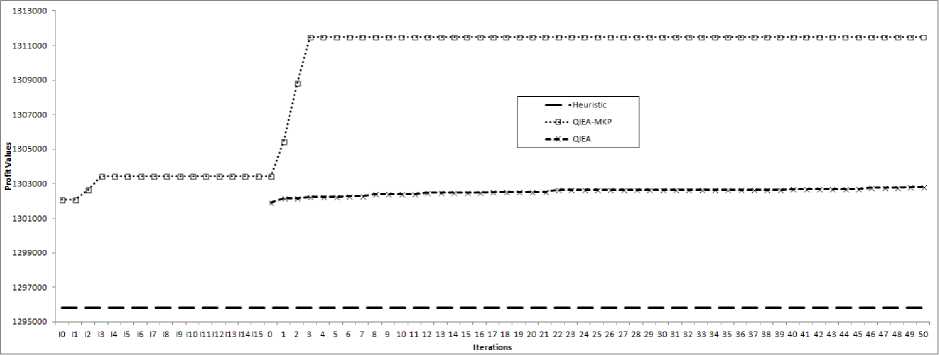
Fig. 7. Comparing convergence of best value achieved using QIEA and QIEA-MKP (an instance having n=5000, m=100)

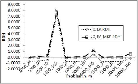
Instances with Similar Capacities

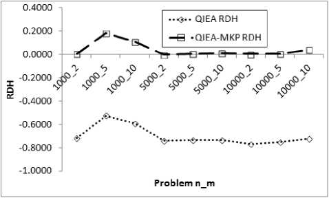
Instances with Dissimilar Capacities

Fig. 8. Comparison of QIEA and QIEA-MKP on the basis of RDH

Instances with Similar Capacities

Instances with dissimilar capacities

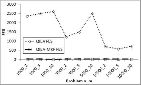
Fig. 9. Comparison of QIEA and QIEA-MKP on the basis of FES required reaching their best solution.

Figures 8 and 9 present a comparison of QIEA and

QIEA-MKP on the basis of quality of solutions and computational effort. RDH of the solutions obtained using QIEA and QIEA-MKP with respect to size of problem instances having different classes of capacities considered is shown in fig 8. Fig 9 plots the Average FES required using QIEA and QIEA-MKP with respect to size of problem instances having different classes of capacities considered.

Following points are observed from the results:

• •    QIEA-MKP shows considerable improvement both in quality of solutions obtained and computational effort required to reach the best as compared to QIEA.

• •    The solutions obtained from QIEA-MKP are much better than the heuristic used to improve solutions locally for most of the instances tested. This improvement is better for instances which required to fill more number of knapsacks.

• •    The hybridised QIEA-MKP is able to provide much better solutions within very less number of FES as compared to QIEA used as the base.

• •    The graph showing quality of solutions with respect to heuristic solution (i.e. RDH) for QIEA-MKP is similar in shape as of QIEA but with a shift from area having solution worse than heuristic to the area having better solution than heuristic.

• VII. C ONCLUSIONS

The QIEA is improved by embedding within it the local improvement based on a known effective heuristic for MKP with an objective to improve exploitation. Apart from it some techniques viz. mutation of solutions appearing to be close to local optima, and reinitializing qubit individuals found incapable to generate new solutions are also induced in order to improve the power to explore the search space. This way the proposed QIEA, with balanced power of exploitation and exploration of search space, provide significantly better solutions with respect to both the QIEA used as base and the heuristic used for proposed hybridization. The proposed QIEA provide better results using much reduced computational effort than basic QIEA.

A CKNOWLEDGMENTS