Beampattern for Multiple Antennas in Hybrid Terrestrial Satellite Communications System (HTSCS)

Published Online October 2013 in MECS

The urge for strong global and reliable connectivity has put considerable pressure on the networks. In order to deal with this problem, stand-alone terrestrial systems are not able to cope up with this problem as the infrastructure is not completely deployed. On the other side satellite systems cannot fulfill this need on their own as the satellite signals cannot penetrate into densely populated areas [5-6]. This problem motivates the location based and demand based hybrid architecture in which the end users can have the facility of terrestrial systems in urban locations as well as can also be served with satellite links when they move to densely populated areas [7]. In such hybrid architecture, terrestrial and satellite networks can share a portion of spectrum which results in low cost and throughout connectivity resulting in increase in system capacity. End user should be transparent of the service provisioned, means that the end terminal should be able to work with terrestrial links as well as with the satellite links. In order to provide such transparent service there is need for a satellite with powerful receiving end so it makes sure that the link margin is up to required level.

This systems provide high data rate, all time connectivity, wide area coverage and significant increased capacity but on the other side of the picture, use of same spectrum by both the satellite networks as well as the terrestrial networks induces sever CoChannel Interference (CCI) [1]. This CCI is main barrier to the achievement of high capacity. In hybrid systems the interference from the mobile to satellite link is dominant hence defines the performance of the system.

Following the sequence of this paper, Section 2 deals with the beamforming and the techniques involved in beamforming. It also encloses the Post/Pre FFT techniques. Section 3 is the system model and performance, which encloses all the simulation results. Section 4 encloses the conclusion and future work.

• II. Beamforming

• 2.1.    Beamforming and Spatial Filtering:

Beamforming is a signal processing technique which is used to control the directionality of the signal in a transducer array either transmitted or received. With the use of beamforming the majority of the signal can be directed in a particular direction from a group of transducers for example radio antenna, audio speaker etc. The term “beamforming” is derived from the fact that early age spatial filter were designed in way to generate pencil beams [8-9]. So it gets clearer that beamforming points to the radiation of signal energy. Beamforming can be applied to either radiation of energy or reception of energy. But in this paper we will use receive side beamforming that is for reception.

The systems which are designed to receive spatially propagating signal usually face the interferers signal. And if the desired signal and interferer signal have the same temporal frequency then it is in vain to use temporal filtering to separate the signals that are desired and interferer [10-12].

In this section we are first going to discuss the operation of beamforming and then will have a look on spatial filtering.

Figures (1) & (2) shown below represent two types of beamformers. The first beamformer shown in fig. (1) is used to process narrowband signals, by sampling the propagating wave field in space. y (k) is the output at time k which is the linearly combined data at sensor

^y ( k ) ^{= X}J ^J - 1 ^wi ^{β x}i ⁽¹⁾

Where w ^β is used to represent the complex conjugate. Conventionally multiplication of data with its conjugate simplifies the notation. Also it is assumed that the data is complex however in many applications make use of quaderature receiver to generate quaderature and in phase data which is termed as I and Q data. As the beamforming is performed digitally so each sensor is assumed to have the required receiver and analogue to digital (A/D) convertor [13-14].

Array Elements

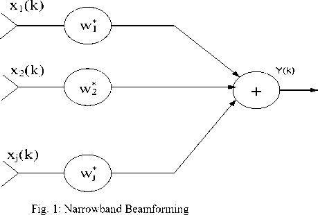
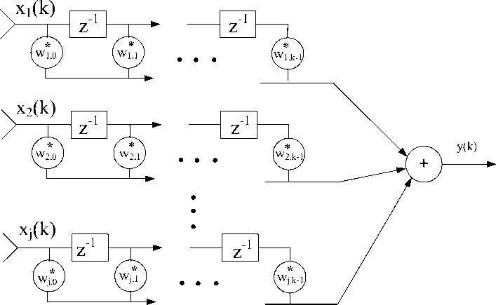
Fig. 2: Broadband Beamformer

Fig. (1) and (2) show the beamformer which is used when a signal of specific frequency is required. It samples the wave field in space as well as in time. The output of the beamformer is as follows

У ( k ) = X i - 1 X k = 0 w f x ,                      (2)

Where, the number of delays in every j sensor is given by K-1 . Taking the signal as an input to each of the sensor represents the beamformer as a multi-input single output.

It’s more suitable to develop a notation which allows treating both the beamformers at the same time. Equation (1) and (2) can be written as by carefully defining the weight w and the data x ( k ) vectors.

H

Y ( k ) = w x ( k )

where H is the Hermitian transpose. If w and x (k) are assumed N-dimensional, it then implies that N=KJ when referring to (2) and in case of (3) N=J. Except the section of adaptive algorithm, time index will be dropped and its presence is assumed understood. So (3) can be rewritten as

Frequency response of an FIR filter with tap weights w ^B p 0 ≤ p ≤ J and tap delay of T seconds is expressed as

r ( w ) = x p = 1 w P jwT                        ⁽⁵⁾

Other way to represent is r^_w ^ = W H dw

Where w^H = w ^ w ^...... w ^

And dw = 1.ej,weJ2wT...,eJ™w

It shows the filter response to the frequency (ω) of a complex sinusoid. The term d (ω) describes the phase of the sinusoid for every tap in FIR filter.

Likewise, the response of the beamformer can be defined as the phase and amplitude fed to a complex wave and making it a function of frequency and location. Generally location is a three dimensional parameter. But we are interested in one dimensional or two dimensional direction of arrival (DOA) [15]. Figure (3) shows how a propagating signal is sampled by an array of sensors.

y = wH x

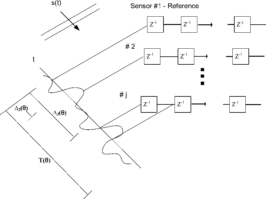
Fig. 2: Sampling of signal from a source located at DOA θ

Figure (3) represents an array which is attached with the delay line that spatially samples the propagating signal. Figure (3) shows the sampling of incoming wave from a source which is located at DOA θ. As there are J samples shown in fig (3). So with K samples per sensor or antenna element, at a time instant is the signal is sampled as N=JK. T(θ) is the duration of time from the very first sample of the first antenna element to the last sample of the last element. And ∆ I ( θ ) is the time delay of the wave arriving between first antenna element (taken as reference) to the last antenna element which is J.

Assume a complex plane wave originating from a source located at DOA θ and ω is the frequency of the signal. For the ease we assume the at the first sensor or antenna element the phase is zero. This results in x = ejωkand x1 = ejω ( j(θ))and for 2 ≤ I ≤ ∆I (θ), where ∆I (θ) is the time delay as described above. So substituting the results in (1) gives us jwk j k=1 β jwΛj(θ)

^y ( k ) ^{= e X}I = 1 ^Xp = 0 ^wp ^{e (6)}

Where ∆1(θ) =  0.r(θ, ω) is the response of the beamformer and it can be expressed as

r ( θ , ω ) = w d ( θ , ω ) (7)

Elements of d(6, to) are correspondent to complex exponential that is ejw j(θ) . Generally it can be stated as jωt1θ  jωt2θ

( θ , ω ) =   . e e

e . j ω t_n θ

Where τ θ , 2 ≤ i ≤ N is the time delays for different taps from the reference point to the point where i t weight is applied. d (9, to) is known as the array response vector and also known as the steering or direction vector. Characteristics of non-ideal sensors may be included in d (9, to) by multiplying each phase shift with a function a i (θ, ω) which depicts the related sensor response as function of direction and frequency [16].

Equation (6) gives the suggestion of vector space understanding of beamformer. This is useful for design and analysis of beamformer [17]. w being the weight vector and d(6, to) being the array response vector is in N dimensional vector space. The response r(θ, ω) is determined by the angle between w and d(6, to). Let’s suppose for (6, to) if the angle between w and d(6, to) is 90o that is there is orthogonality between w and d(6, to), then zero will be the response in this case. And on the other hand if the angle is zero or close to zero then the response will be maximum of near to maximum. So in order to distinguish between different sources at different locations and/or frequencies; let’s say (θ1, ω1) and (62, to2) is calculated from the angles between d(61, to1) and d(62, to2) which are their array response vectors [18-19].

• 2.2.    Adaptive Algorithms for Beamforming:

• 2.3.    Least Mean Square (LMS):

Adaptive or smart antenna arrays are used to achieve the adaptive beamforming [18]. In order to achieve this task the weights of the antennas elements are adjusted in such a way so as to suppress the interference which is caused form the undesired users, as a result the desired signal is enhanced. The term that categories the adaptive beamforming algorithm is their convergence property and complexity in computation.

There are different adaptive algorithms which are used in adaptive beamforming e-g Sample Matrix Inversion (SMI), Recursive Least Square (RLS), Least Mean Square (LMS) etc. But for this paper LMS is of interest which we will be using in beamforming.

The reason of using LMS is its simplicity and its suitability  for continuous data transmission  [20].

Although LMS algorithm slowly converges when compared to more complicated algorithms like RLS [21] but it is simpler to implement. Unlike SMI, the LMS does not invert the covariance matrix directly [22].

Suppose an adaptive beamformer which uses a Uniform Linear Array (ULA). The response of the beamformer at the output is

T

^y ( n ) ^{= wn x} ( n )                                   ⁽⁸⁾

In (8) “w” is the array weight vector which is associated to N-element array, x is the signal vector received at the beamformer input. Initializing of array weights vector in a standard LMS algorithm is done arbitrarily and then it is updated using LMS equation

w(n+1) =wn +µdnwnxn                     (9)

In (9) X (_n) is the nth sample of the desired signal at nth iteration, where d (_n) is desired signal and ц is known as the step size which controls convergence rate of the beamformer [23]. This step size controls that how quick the algorithm attains the steady state. Smaller the value of μ , the longer it will take to converge to a steady state; this means that it would need long training sequence to converge. In order to get the clear idea of the algorithm a simple block diagram is shown in fig. (4).

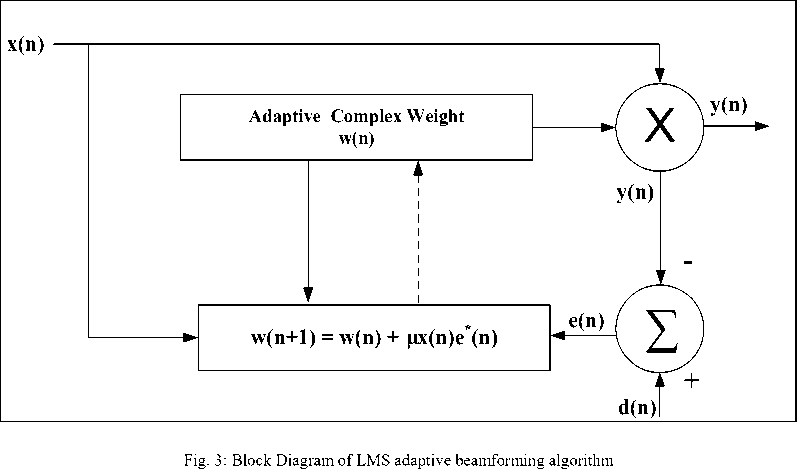
Noticing (9), LMS algorithm need to have the knowledge of desired signal d(n). It can be achieved in a digital system by transmitting a data that is known to receiver, known as training sequence or pilots. Since in a standard LMS algorithm the weights are arbitrary initialized, it can take longer to reach convergence state because the weights initialized in the start might not be similar to final solution.

• 2.4.    Beamforming Techniques for OFDM system:

For OFDM systems, beamforming techniques can be divided into two categories,

• >    pre- Fast Fourier Transform (pre-FFT) beamforming

• >    post-Fast    Fourier    Transform    (post-FFT)

• 2.5.    Post-FFT Beamforming:

beamforming.

The pre-FFT is in done in time domain [22, 23], while post-FFT is done in frequency domain [23-24].

Post-FFT beamforming is done in frequency domain. It is also termed as frequency domain beamforming because all the array processing is carried out after the FFT that is when the signal is transformed from time domain into frequency domain. For this post-FFT will be requiring set of weights for each antenna array so that the processed weights should be equal to the antenna elements times the subcarriers. But this process involves complex computation. Figure (5) explains the post-FFT scheme [24].

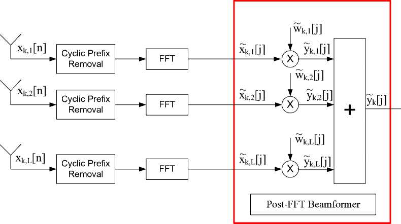
Fig. 4: Post-FFT beamforming scheme

In fig. (5) a method for post-FFT is presented and it’s quite clear that it requires FFT blocks of length L which means that one FFT block for one antenna as discussed above. And the beamforming is applied after the signal is transformed into frequency domain. Here in this scheme the frequency samples x_k,L[j] are multiplied with different weights w k,h [j] where j represents the index of frequency. After the multiplication all the data is summed up resulting into y k [j] which is the desired user data and is ready to fed to demodulator.

In post-FFT as well in pre-FFT (see later) weights are calculated by reducing the Mean Square Error (MSE). A reference signal is required in order to start calculating MSE; it can be done either by providing preamble [25] which is transmitted periodically or by using pilots.

• 2.6.    Pre-FFT Beamforming:

Beamforming is an interference mitigation technique which is used to extract the desired signal from other interferer signals provided they are using same frequency but have different location. Interference can be caused by undesired signals or it can be induced from the multipath environment [26]. So pre-FFT beamforming also termed as time domain beamforming is used to extract the desired signal from the interferer signal and it is done in time domain that is before the operation of FFT as shown in the fig. (6).

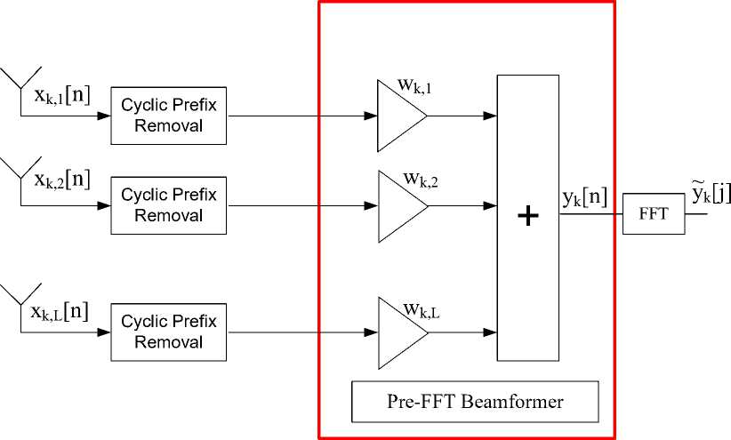
Fig. 5: Pre-FFT beamforming scheme

From fig. (6) it is quite obvious that pre-FFT beamforming can be broken down into two steps. In first step the signal is received at the beamformer input and in the second step weights are calculated and are applied to the received signal.

Figure (6) represents the beamforming scheme in which x_k,L[n] are the received signals at the beamforming input. After passing through block of cyclic prefix removal these received signals are then multiplied with the weights ( w_k,L ) calculated from adaptive beamformer algorithm as we have already discussed above. Then is the process of summation and the desired extracted signal ( y k [n] ) is received at the output of the summation block. And [n] here shows the time domain.

• ^y ( n ) ^{= x}k ^M = 1 ^wk^xk , L ^{= w H x}L ⁽¹⁰⁾

Here the subscript H shows the Hermitian, which is the complex conjugate transpose of the vector where as w is the array weight vector.

w = (w , w ,......w )T x = (x n,x n,.....xkn)T where T is the transpose of the vector, the system output can be notified as

• yn = wHxn                              (11)

In order to obtain the output of the array, multiply the coming signal with its respective weight. In order to perform it in vector notation, simply take the inner product of both the vectors which are weight and signal vector as shown in (11).

The pre-FFT beamforming technique is easy to implement as it shows simplicity in its architecture and also in computational cost [23-27]. Whereas post-FFT when compared with pre-FFT shows better performance but it involves more implementation complexity. So we trade off degradation in performance with less computational complexity.

• III.    Simulation Results

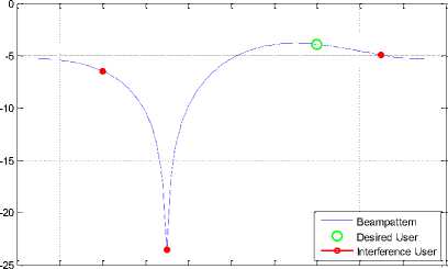
Here in this section we will look upon the beampattern generated from the results presented above. The beampattern will give a clearly insight about the beam which is directed towards the desired user and nullifying the effect of interference.

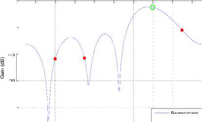
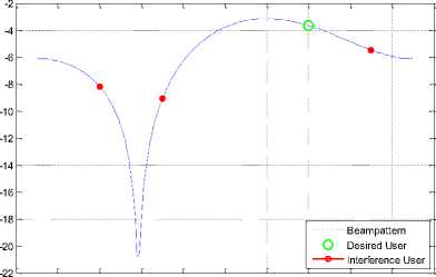
Before proceeding things which should kept in mind are the desired user position which is located at 40 degrees and three interferer users which are located at -60, -30 and 70 degrees. Let’s start with the first scenario where interference level is -10dB

-100    -80     -60     -40     -20       0      20      40      60      80      100

Azimuth (θ)

Fig. 7: Beampattern for BPSK for 2 antenna elements

One thing to note here is that although the interferers are not getting their nulls properly and this is just because of small number of antenna elements.

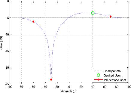
Fig. 9: Beampattern for QPSK for 2 antenna elements

-5

-10

-15

-20

-25

Beampattern

Desired User о Interference User

-30 t---------------[---------------с---------------[---------------с-------------- 'I               I               I             Ч

-100     -80     -60     -40     -20       0       20      40      60      80      100

Azimuth (θ)

Fig. 10: Beampattern for QPSK for 4 antenna elements

-5

-10

-15

-20

-25

Beampattern

Desired User о Interference User

-30

-100    -80     -60     -40     -20       0      20      40

Azimuth (θ)

80     100

Fig. 8: Beampattern for BPSK for 4 antenna elements

Figure (7) and (8) show the Beampattern for modulation scheme BPSK with 2 and 4 antenna elements respectively. The desired user is located at 40 degrees, and interferes are located at the position mentioned in fig. (9). It gives more clear view of the beam directed towards the desired user.

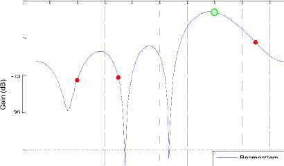
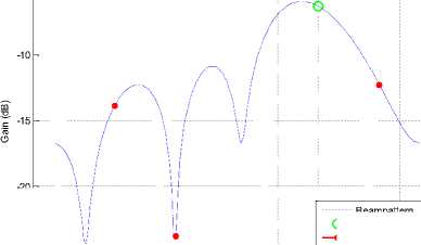
Figure (9) and (10) show the Beampattern for modulation scheme QPSK using 2 and 4 antenna elements. Again similar pattern as we have seen for the case of BPSK. But as the antenna elements have increased from 2 to 4 there is a different of around 5 dB between the desired user n interferer users.

-2

-4

-6

-8

-10

-12

-14

-16

-18

-20

Beampattern

О Desired User

Interference User

• -22 t---------------(---------------с---------------(---------------(---------------с---------------(-------------- 'I               I               I             Ч

  -100     -80     -60     -40     -20       0       20      40      60      80      100

Azimuth (θ)

Fig. 11: Beampattern for 8-PSK for 2 antenna elements

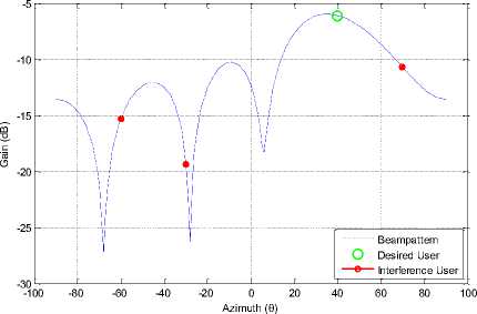
Fig. 12: Beampattern for 8-PSK for 4 antenna elements

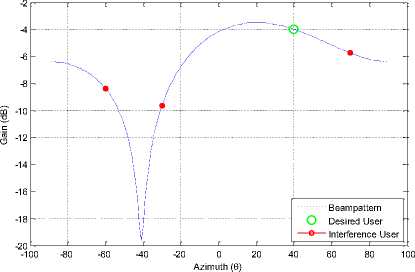
Fig. 15: Beampattern for QPSK for 2 antenna elements

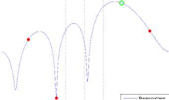
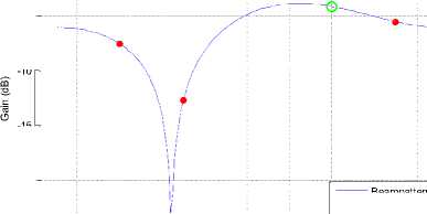
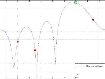
One thing very interesting to note here that changing modulation scheme does not put any significant effect on beampattern. But when the antenna elements are changed beam pattern changes along with.

In the second scenario the power of the interferer users is -5dB.

-5

-10

-15

-20

-25

Beampattern

Desired User

—е— Interference User

-30

-100     -80      -60      -40      -20       0       20

Azimuth (θ)

-5

-10

-15

-20

Beampattern о Desired User

—э— Interference User

-25

-100    -80     -60     -40     -20      0      20

Azimuth (θ)

Fig. 16: Beampattern for QPSK for 4 antenna elements

-6

Fig. 13: Beampattern for BPSK for 2 antenna elements

-8

-10

-12

-14

-16

-18

-20

-22

-24

Beampattern о Desired User

Interference User

-26

-100    -80     -60     -40     -20       0      20

Azimuth (θ)

-100    -80     -60     -40     -20      0      20     40      60      80     100

Azimuth (θ)

Fig. 17: Beampattern for 8-PSK for 2 antenna elements

80     100

Fig. 14: Beampattern for BPSK for 4 antenna elements

-5

-20

Fig. 18: Beampattern for 8-PSK for 4 antenna elements

Beampattern

Desired User

Interference User

-25

-100     -80      -60      -40      -20       0       20

Azimuth (θ)

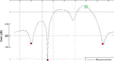
In order to see the variation of the Beampattern in accordance with increase in number of antenna element, a very interesting example is modelled here. In this case, 6 antenna elements have been used to study the effect of increasing the number of antenna elements on the system. Also the main aim of using large number of antenna is to avoid interference by placing the interferers at nulls. In this example 6 antenna elements are used along with all the modulation schemes.

-5

-10

-15

-20

-25

-30

Beampattern о Desired User

—э— Interference User

-35 t____________[____________[____________[____________[____________[____________[_

-100    -80     -60     -40     -20       0      20

Azimuth (θ)

Fig. 19: Beampattern for BPSK for 6 antenna elements

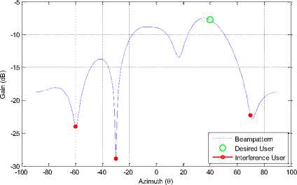
Fig. 20: Beampattern for QPSK for 6 antenna elements

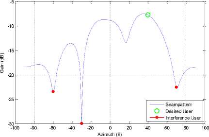
Fig. 21: Beampattern for 8-PSK for 6 antenna elements

It is clearly observed from fig. (19), (20) and (21) that the interferer users are placed at the nulls and desired user is getting the maximum gain.

• IV.    Conclusion and Future Work

The issue raised in this paper is successfully achieved. The results are evaluated fairly.

After going through the results and simulations we have come to know that the system performance increases with the increase in energy but decreases when higher order modulation schemes are used. For this 4 modulation schemes are evaluated in single and multiuser OFDM implementation and 3 modulation schemes are implemented for OFDM system with beamforming. The results of the beamforming shown in fig. (8) represents the improvement in the performance with increasing the bit energy. As different modulation schemes are compared so energy per bit metric is used to establish a fair comparison between them instead of signal to noise ratio.

Also going through the subsequent figures, it is noticed that when the number of antenna elements are increased the system performance improves. Performance of the system with 4 antenna elements out performs the system with 2 antenna elements. But increasing the number of antenna elements increases the payload of the satellite which impacts the weight of the satellite, its power consumption etc. Figures (19), (20) and (21) show the beampattern of six antenna elements and it is clear that the interferer users are placed completely at their nulls and the desired user is getting the maximum gain. This is because the weights used for the data extraction are close to optimal. As the dimension of the array response depends upon the number of antenna elements so the data is extracted with more precision. So it is obvious that increasing the antenna elements increases the system performance.

Another scenario is depicted in fig. (11) in which the interference power is increased to -5 dB per user. Comparing the results of fig. (11) with those shown in fig. (12) in which interference power was -10 dB shows the performance degrades with the increase in interference power.

In order to carry out future work relating to this paper, is its implementation relating to 3GPP. This paper has also been simulated with a 3GPP standard using 256 subcarriers with pilot transmission every 6th subcarrier [27]. But in this work staggering is not done. So this work can be extended to the next level by staggering the pilots in time and frequency domain and then analyzing the impact on the system performance.

Also the work done in the paper can be extended further where Post-FFT beamforming technique can be implemented instead of Pre-FFT beamforming as done in this paper. A fair comparison can be evaluated on the basis of these two adaptive beamforming techniques.