Bezier Curves Satisfiability Model in Enhanced Hopfield Network

Published Online December 2016 in MECS

Computer Aided Geometric Design (CAGD) has emerged as one of the most eminent fields in computer graphic, numerical computation, and geometrical studies. The renaissance of CAGD is inaugurated by the various form of Bezier curves that has attracted a prolific number of research [1]. Hence, Bezier curves are one of the most intensively used in CAGD [2]. Popularized by Bezier [3], Bezier curves are used to construct smooth curves at any scale by considering its own properties to be applied in the design. The main impetus of this research is to reconstruct the Bezier curves according to the correct properties by using neural network approach. Hence, the Bezier properties verification process requires a robust and stable algorithm in order to construct more complex

Bezier curves. Thus, we choose to translate the Bezier curves properties into 2-Satisfiability problem and integrate it in Hopfield neural network by using logic programming (HNN-2SAT). Basically, 2-Satisfiability (2SAT) is the prominent counterpart of the Boolean satisfiability (SAT) optimization problem, that is denoted in Conjunctive Normal Form (CNF) form [4, 8]. Without a doubt, there have been a lot of applications of 2-Satisfiability such as the previous work by Femer [5], Papadimitriou [6], Patreschi and Simeone [7]. These related works emphasized on the 2-Satisfiability as an optimization problem. On the separate note, we can transform any real dataset or mathematical p roperties into 2SAT form with the assistance of logic programming [9]. In this paper, we emphasized on the Bezier curve properties as 2SAT combinatorial optimization problems in logic programming.

The Hopfield neural network plays an important role in the field of artificial intelligence and mathematical computation. Recurrent Hopfield neural networks are principally dynamical schemes that feedback signals to themselves. The network was inaugurated by Hopfield and Tank [10]. One of the interesting features is the network possess a dynamical system with stable states with each own basin and attraction [11]. Moreover, the Hopfield neural network minimizes Lyapunov energy because of physical spin of the neuron states. On top of that, the network produced global output by minimizing the network energy. Gadi Pinkas and Wan Abdullah [9, 12] demarcated a bi-directional mapping between logic and energy function of a symmetric neural network. Besides, both related works are the building blocks for a corresponding logic program. The work of Sathasivam [13] presented that the optimized recurrent Hopfield network could be possibly used to do logic programming. Above all, the ability of learning by using Hopfield network is the main priority in the reconstruction of the Bezier curves. The memory will be stored in Hopfield’s brain as content addressable memory (CAM) [14]. Hence, we can reconstruct the correct Bezier curves by retrieving the stored memory based on the properties.

Logic Programming refers to an auspicious field, and widely used to resolve numerous constraint optimization problem [15]. Additionally, the logic programming can be demarcated as an optimization problem [13, 16]. In this paper, the Bezier properties will be represented by the clauses in 2SAT. After that, 2SAT problem will be translated into logic programming integrated with Hopfield neural network. The impetus of our study is the well-known Wan Abdullah’s technique [9, 12]. Wan

O ( l .2 n ) operations [28] and it was proven by many that SAT is an NP-complete problem.

SAT problem normally represented in Boolean variables or expressions in conjunctive normal form (CNF). CNF is defined as conjunction of clauses, where the clauses are disjunction of literal [35]. Literal is a variable or its negation. For example:

( x 1 V x ₂ ) л ( — x ₂ V x ₃ V— x 5 ) л ( — x 1 V x 4 )        (1)

Based on (1), x , x , x , x are Boolean variables to be assigned, — means negations (logical NOT), v means negations (logical OR), л means negations (logical AND). We can satisfy formula (1) by taking x = true , x ₂ = false , x ₃ = false , x 4 = true . However, if any formula is not satisfiable, it will be termed as unsatisfiable.

In Bezier model reconstruction, we integrate the foundation of satisfiability in order to obtain the correct Bezier model. The literals in every clause will be represented the properties of the Bezier curve model.

• A. 2SAT

2SAT is a subset of SAT problem. It is a classical NP-problem that determine the satisfiability of sets of clauses with at most two literals per clause (2-CNF formulas) [8]. Besides, it is popular and highly regard problem for general Boolean satisfiability which can involve constraints on two variables [31]. In addition, the variables can allow two possibilities for the value of each variable. 2SAT problem can be expressed as 2-CNF (2-Conjunctive Normal Form). Randomized 2SAT problem is considered as NP problem or non-deterministic problem [6]. The three fundamental components of 2SAT are summarized as follows:

• 1.    A set of m variables, x , x ,......, x

• 2.    A set of literals. A literal is a variable or a negation of a variable.

• 3.    A set of n distinct clauses: C , C ........C . Each clause consists of only literals combined by just logical OR ( ^V ). Each clause must consist of 2 variables.

The Boolean values are {1,-1} . Researchers have replaced F and T in the neural networks by 1 and -1, respectively to emphasized false and true. Since each variable can take only two values, a statement with n variables requires a table with 2n rows. The goal of the 2SAT problem is to determine whether there exits an assignment of truth values to variables that makes the following Boolean formula P satisfiable.

n

P =л C i                  (2)

I = 1

Where л is a logical AND connector. Ci is a clausal form of DNF with 2 variables. Each clause in 2SAT has the following form

n

^Ci ⁼ ^ ( x i , y )

x i e { k i , — k i } and y, e { r i , — r i } — k i and — r i are negations of the literals.

• III.    B EZIER M ODEL S ATISFIABILITY

Popularized by French engineer, Pierre Bezier, Bezier curve is a parametric curve that frequently used in computer graphics and design automobile bodies. Currently, Bezier curves are extensively used to model smooth curves and other applications [20]. A Bezier curve is defined by a set of control points P ₀ through P _n , where n is the order of the curve. In essence, the first and the last control point are always the end point of the curve. The other point between the first control point to the last do not lie on the curve [21]. Since the curve is completely enclosed in the convex hull of its control points, the points can be manipulated graphically.

• A.    Properties of Bezier Curve

Bezier curve is a parametric curve that uses the Bernstein polynomials as a basis. Generally, a Bezier curve of degree n (Order n+ 1) is represented by

n

B ( t ) = Z b i,n ( t ) P i ,  0 - t - 1        (4)

i = 0

where

( П b,n (t) = l    Iti (1 -t)n i , n = 0,1,2,3,.....,n         (5)

The shape of the curve can be determined by using the coefficient P i which are the control points and B in ( t ) are the basis of the function [21]. Lines can be drawn between the control points of the curve in order to form control polygon. Bezier curve possessed the following properties

• 1)    Geometry invariance property:

Partition of unity of the Bernstein polynomial satisfy any of the Bezier curve although the curve undergoes translation and rotation of its control point [22].

The basis function of any Bezier curve can be represented by using the following graph:

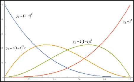
Fig.1. Basis function for cubic Bezier

• 2)    Geometric point property:

• (i)    The first and the last control points are the endpoints of the curve. Moreover, b₀ = B ( 0 ) and b n = B ( 1 ) .

• (ii)    The curve is a tangent to the control polygon at the endpoints [21]. This can be verified by taking first derivatives of a Bezier curve

dB ( t )    n -L

B ( t ) =  ^   = n £ ( P i + 1 - P i ) b i , n - 1 ( t ) ,  0 - 1 - 1  (6)

i = 0

In detail, we acquire    P ' ( 0 ) = n ( P 1 - P₀ ) and

B ' ( 1 ) = n ( P; - P ;-1 ) . The above equation can further simplified by setting A P = P ₊₁ - P :

n - 1

B ' ( t ) = n ^ A PB i , n - 1 ( t ) ,  0 - t - 1           (7)

i = 0

• 3)    Convex hull property:

A domain D is considered as a convex if an y t wo points P and P in the domain, the segment P ₁ P ₂ is entirely embodied in the domain D [23] . The convex hull of a set of points P is the boundary of the smallest convex domain containing P. The entire curve is contained within the convex hull of the control point.

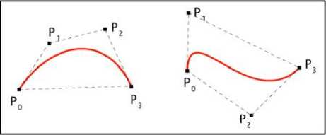
Fig.2. Convex hull built from the control point

• B.    Type of Bezier Curve

A Bezier curve is defined based on their control points. For our studies, we will examine the following curve

• 1)    Linear Bezier curves

Given points P and P , a linear Bezier curve is a straight line between those two points. The curve can be formulated as followed

B (t ) = (1-t) Po + tP            (8)

Where 0 <  t <  1 .The equation normally similar to linear interpolation.

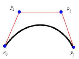
Fig.5. Cubic Bezier curve

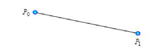
Fig.3. Linear Bezier curve

• 2)    Quadratic Bezier curves

Quadratic Bezier curve is a curve that traced by the function B ( t ) given points ? 0 , P and ? 2 . The curve can be formulated as followed:

B ( t ) = ( 1 - 1 ) ² P 0 + 2 ( 1 - 1 ) tP + 1 ² P ₂ (9)

Where 0 <  t <  1 . The equation is interpreted as the linear interpolant of corresponding points on the linear Bezier curves from P ₀ to P ₁ and from P ₁ to P ₂ [24].

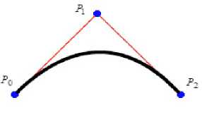
Fig.4. Quadratic Bezier curve

• 3)    Cubic Bezier curves

Cubic Bezier curve is a curve that traced by the function B ( t ) given points P 0 , P , P 2 and P 3 . Cubic Bezier curve can be formulated as followed:

B ( t ) = ( 1 - 1 ) ³ P ₀ + 3 ( 1 - 1 ) 2 tP 1 + 3 ( 1 - 1 ) t ² P 1 + 1 ³ P ₃ (10)

Where 0 <  t <  1. The curve will not pass through P or P ₂ because these points only to provide directional information. The cubic Bezier curve can be defined as a linear combination of two quadratic Bezier curves [25].

C. Bezier-SAT

Table 1. Bezier-2SAT clause representation

Clause	Properties	Descriptions
C 1	Partition of unity n E B in ( t ) = 1 i = 0	Linear Bezier C 11 = ( 1 - 1 ) C 12 = t Total clauses: 2 Quadratic Bezier C 11 = ( 1 - 1 ) 2 C 12 = 2 ( 1 - 1 ) C 13 = t2 Total clauses: 3 Quadratic Bezier C 11 = ( 1 - 1 ) 3 C 12 = 3 ( 1 - 1 ) 2 C 13 = 3 ( 1 - 1 ) t2 3 C 14 = t Total clauses: 4
C 2	Geometric point where P are the control points of the curve. The curve must touch the first and the endpoint.	C 21 = P 0 C 22 = P 1 C 23 = P 2 C 24 = P 3 C 2 i = P - 1 Total clause: i - 1
C 3	Convex hull property	{ P 0 , P , P 2 , P 3,..... , P i H Where D is the domain of the convex hull Total clause : i - 1

The properties of Bezier curve with different orders can be represented by using logic. In this case, 2SAT logic is utilized to implant the important properties of Bezier curve. If any of the random curve followed all the important properties of Bezier curve [25], the curve model is considered as Satisfiable (It is a Bezier curve). On contrary, if any of the curve model does not abide with properties, 2SAT logic will consider the curve as unsatisfiable (It is not a Bezier curve) [26]. The task of representing the important properties of Bezier curve in 2SAT will be used in training phase of neural network. It was proven by previous researchers that the hybridization between 2SAT logic and neural network is able to solve constraint optimization problem such as pattern reconstruction. Table 1 shows the representation of the properties of the Bezier curve and 2SAT clause during training phase.

• IV.    B EZIER -SAT IN H OPFIELD N EURAL N ETWORK

Neuro-logic is the blend of neural network and logic programming as a single hybrid network. Specifically, the neuro-logic methods can be applied in a various field such as constraint optimization problem, pattern recognition, circuit and curve reconstruction [33]. In this paper, we apply the Hopfield neural network and logic programming to reconstruct the Bezier curves according to the properties needed based on 2SAT instances. The effectiveness of our proposed paradigm (HNN-2SAT) will be discussed briefly in Section VI.

• A.    Hopfield Model

In Bezier curve reconstruction, we select the Hopfield neural network because it is well distributed. Hence, Hopfield neural network is easier to be integrated with any paradigms to solve satisfiability problem [31].

Technically, we incorporate the 2SAT with 3 clauses in Hopfield neural network so that we can relate it with the Bezier curve properties. The correctness of Bezier curve that will be reconstructed totally rely on the effectiveness our proposed network. In addition, the Hopfield neural network can be demarcated as a model of content addressable memory (CAM) [15, 16]. In layman’s term, we call it as Hopfield’s brain. Hence, Hopfield’s brain replicates our biological brain function to store and process the memories. Besides, the learning and retrieving data in Hopfield neural network are the fundamental aspect of content addressable memory (CAM) [11, 14].

Specifically, the Hopfield neural network is a class of recurrent auto-associative network [33]. The units in Hopfield models are predominantly binary threshold unit [34]. Hence, the Hopfield nets will yield a binary value such as 1 and -1. The definition for unit I’s activation, a _i are given as follows:

a i = *

' 1 if E W J ^

-1 Otherwise where Wij is the connection strength from unit j to i . Sj is the state of unit J and ^ is the threshold of unit i . The connection in Hopfield net typically has no connection with itself Wit = 0 and connections are symmetric or bidirectional [12, 13].

Hopfield network work asynchronously with each neuron updating their state deterministically. The system consists of N formal neurons, each is described by an Ising variable. Neurons are bipolar St e{1, —1} obeying the dynamics S; ^ sgn(h ) where the local field hi . The connection model can be generalized to include higher order connection. This changes the field to hi=E Wj2 Sj + Л° (12)

The weight in Hopfield network is always symmetrical. The weight in Hopfield network denotes to the connection strength between the neurons. The updating rule maintains as follows:

S i ( t + 1 ) = sgn [ h ( t ) ] (13)

This property guarantee the energy will decrease monotonically even though following the activation system [14, 30]. However, it will drive the network to search for the possible minimum energy. The following equation represents energy for Hopfield network.

E = •••• — 1 EE w j ²⁾ S i S j — Y W⁽¹⁾ S j (14) iji

This energy function is vital to improve the degree of convergence of the proposed network [18]. Thus, the energy value is important to obtain global Bezier curves. The power of reconstructing the curves depends on how the synaptic weights are computed. Hence, our proposed networks are able to update the weights and proceed the Bezier curves reconstruction effectively.

• B.    Logic Programming in Hopfield Network

Implementation of HNN-2SAT in Logic Programming.

• i.    The 2SAT clauses are transformed into Boolean algebra. Thus, the clauses will form a formula that will be used to check the properties of Bezier curves. In this paper, each clause represents the properties of the Bezier curve.

• ii.    Identify a neuron to each ground neuron. Then, initialize all the possible weights to zero.

• iii.    Derive a cost function with negation of all 2SAT clauses. As an illustration, we have the following cost

  functions,

  
  

X = 1 (1 + S ) and X = 1 (1 - Sx ) .

Hence,

the states are represented as   S x = 1 (True) and

S x = - 1 (False). For this scenario, the multiplication signifies conjunction and addition symbolizes disjunction.

• iv.    Comparing the cost function with energy, E by obtaining the values of the connection strengths. (Wan Abdullah’s Method) [9]

• v.    Check clauses satisfaction by using exhaustive search. Hence, the satisfied assignments will be stored. In this paper, the satisfied assignments for the Bezier curves (correct properties) will be stored as content addressable memory (CAM).

• vi.    The states of the neurons are randomized. The network undergoes sequences of network relaxation [14]. Calculate the resultant local field h_t ( t ) of the state. Let say if the final state is stable for 5 runs, we consider it as final state.

vii. Compute the corresponding final energy E of the final state via implementing Lypunov equation. Authenticate whether the final energy achieved is a global minimum energy or local minima. In Bezier curves reconstruction, the final energy depicts the correct properties of the Bezier curves. Finally, the global Bezier model and running time are computed for every Bezier models.

• V.    I MPLEMENTATION

  In this exploration, we require methodical procedures. The procedures would work by using Microsoft Visual C++ 2013 as a platform to simulate our logic program. First of all, we generate a random program based on 2SAT clauses. In Bezier curve reconstruction, we represent each of the properties of Bezier model as the clauses. Each of the clauses form randomized 2SAT formula. Each of the clauses consist of the randomized state. The states of the 2SAT clauses (representing properties of the Bezier) will be verified and the correct clauses will be retained (training stage). After undergo HNN-2SAT, the network reached the final states. Equation (13) is vital to ensure the network achieve stable states. Stable final states will be achieved when the state remains unchanged for 5 consecutive runs. Pinkas [18] emphasized that by permitting an ANN to evolve in time shall lead to the stable state where the energy function obtained does not change further. In this case, the corresponding final energy for the stable state will be calculated. If the difference between the final energy and the global minimum energy is within the termination criteria, then consider the solution as global minimum energy. 0.001 was chosen as a termination criterion since this value gave us better output accuracy. We run 100 training and 100 combinations of neurons in order to reduce statistical error. Since the network will produce 10000 Bezier models, we calculate the percentage of

global Bezier model. Running time will be recorded from the start to the end of the program. In this paper, the global Bezier model is considered as the global solution.

• VI.    R ESULT AND D ISCUSSION

In order to test the performance of HNN-2SAT in reconstructing the Bezier curve model, we evaluated the proposed paradigm based on global Bezier model and running time.

• A.    Global Bezier model

Table 2. Global Bezier model for reconstructed linear Bezier curves

Number of Reconstructed Linear Bezier Curves	Global Bezier Model (%)
20	100
40	100
60	98.3
80	96.7
100	96.2
120	94.9
140	93.7

Table 3. Global Bezier model for reconstructed quadratic Bezier curves

Number of Reconstructed Quadratic Bezier Curves	Global Bezier Model (%)
20	100
40	99.9
60	98.6
80	96.6
100	95.7
120	94.8
140	92.3

Table 4. Global Bezier model for reconstructed cubic Bezier curves

Number of Reconstructed Cubic Bezier Curves	Global Bezier Model (%)
20	100
40	98.9
60	98.0
80	96.1
100	95.3
120	92.5
140	90.8

Table 2, 3 and 4 illustrate the global Bezier model configuration for the different type of curve. Based on the table, we successfully reconstruct the correct Bezier model for all type curves. HNN-2SAT are able to reconstruct 20 Bezier curves (Global Bezier model) for all order of the curve without encountering any nonBezier model (Local Bezier model). The proposed paradigm is able to train the network with the properties of the Bezier via 2SAT and successfully retrieved the correct clause during the reconstruction phase. As the number of reconstructed Bezier curve increased, the complexity of the network increased. Local Bezier models are expected to emerge because the solution of HNN-2SAT trapped at the suboptimal solution. This is due to spurious minima occurred during the retrieval phase and the network recalled the wrong states for the clauses (Bezier properties) [14, 13] Consequently, the existence of local Bezier model will create a curve which does not follow the properties of the Bezier curve. Comparatively, cubic Bezier model produced the highest number of local Bezier curve compared to linear and quadratic Bezier curve. This is because cubic Bezier has more basis and control points compared to linear and quadratic Bezier curve. By the same token, the cubic Bezier constraints embedded in HNN-2SAT will be larger and more complex compared to linear and quadratic Bezier curve. Local Bezier curves are expected to increase if the order of the Bezier curve increased. For example, quartic Bezier curves are expected to produce more local Bezier model compared to cubic Bezier. In general, almost 90% of the curve (linear, quadratic and cubic) produced by HNN-2SAT are global Bezier curve.

• B.    Running Time

Table 5. Running time for reconstructed linear Bezier curves

Number of Reconstructed Linear Bezier Curves	Running Time (s)
20	0.0100
40	0.2600
60	0.5238
80	1.263
100	1.640
120	2.050
140	2.503

Table 6. Running time for reconstructed quadratic Bezier curves

Number of Reconstructed Quadratic Bezier Curves	Running Time (s)
20	0.1500
40	0.2900
60	1.040
80	1.113
100	1.530
120	2.440
140	3.450

Table 7. Running time for reconstructed cubic Bezier curves

Number of Reconstructed Cubic Bezier Curves	Running Time (s)
20	0.2772
40	0.6600
60	1.318
80	1.790
100	2.175
120	3.326
140	4.100

Running time is another measure or indicator to check the effectiveness of our proposed network [15]. Table 5, 6 and 7 depict the running time for our proposed network, HNN-2SAT to reconstruct different Bezier curves correctly. A closer look at the running time indicates that the HNN-2SAT has successfully reconstructed the curves within the stipulated time frame. The running time obtained in this study provides convincing evidence that the time taken for the HNN-2SAT to learn and retrieve the correct curves slightly varies for the different type of Bezier curves. As a matter of fact, the training process consumed most of the running time as our proposed network will be checking the properties of the correct Bezier curves. Strictly speaking, in order to generate the correct Bezier curves, three main properties (constraints) must be fulfilled. Hence, the verification requires particular time to complete the entire process. Theoretically, as the number of Bezier curves model increases, the running time will also increase. In the previous measures, the issue under scrutiny is the existence of local Bezier in any complex model. Table 5, 6 and 7 delineates the significant differences in the running time obtained for the linear, quadratic and cubic Bezier model if the number of curves is ranging from 100 to 140. According to the results, the running time for linear Bezier model is faster than quadratic Bezier, especially when more curves are introduced. Conversely, the cubic Bezier model required more running time. This is due to the cubic Bezier comprised of more basis and control points compared to linear and quadratic Bezier curve. Thus, the training process in order to reconstruct the correct Bezier curve became much slower. There is overwhelming evidence corroborating the notion that more running time required for highly complex Bezier model. A clear evidence is the computation burden to reconstruct higher order curves. Hence, better optimization technique can be applied to improve the running time for highly complex Bezier models. For the time being, HNN-2SAT is still the best network.

• VII.    C ONCLUSION

We have presented our proposed paradigm, namely HNN-2SAT network to reconstruct various Bezier curves model. It had been presented by the computer simulations that our proposed model that incorporated with Hopfield neural networks were able to retrieve and reconstruct correct curves model within the exceptional time frame. Information from the various Bezier models can be stored in the clausal form in Hopfield and most of the retrieved model are exact Bezier models. Hence, the proposed models are supported by the strong agreement of global Bezier model obtained and running time. This early work may have some limitations which will be addressed in future work. Finding satisfied interpretations which have been a building block for clause during simulation can be very complex and detrimental. We have noted that optimized and effective searching technique should be drawn in order to find the correct clausal state. This requires further investigation. For future work, approximation algorithm such as heuristic methods can be implemented in order to find the correct interpretation for clauses. On the separate note, we can consider variety satisfiability logic such as 3-Satisfiability to represent the clauses in Hopfield network.