Big data analytics and visualization for hospital recommendation using HCAHPS standardized patient survey

Published Online March 2019 in MECS DOI: 10.5815/ijitcs.2019.03.01

The digitization of procedures involved in medical diagnosis and healthcare industry produces a tremendous amount of digital data which is capable of deriving sound conclusions for advanced decision making. Patient satisfaction is a quality tool, one of the legit indicators to assess the quality of the Hospitals [1-3]. The surveys recorded from Hospitals and other healthcare centers can be useful for measuring patient satisfaction parameters and present with critical analysis to help the patients and evaluate the overall performance of the hospitals. With the idea to provide a recommendation on the quality of the hospital to the user based on past survey measures of the hospital, we put forward a hospital recommendation system. We propose a multi-disciplinary approach to train a predictive model on HCAHPS (Hospital Consumer Assessment of Healthcare Providers and Systems) dataset for the recommendation of a hospital, based on specific set of features and we also analyze which features significantly contribute to having a good recommendation for a hospital. HCAHPS is a U.S based national survey of hospital patients about their experiences during a recent hospital stay [4]. We utilized the survey data as an asset for deriving Analytics and producing reports via Predictive analysis methods and several Visualization techniques. In previous literature, the use of semantic search for the recommendation of health care has been proposed by various practitioners [5-7], which may not apply to a complex healthcare survey having a large number of characteristics. G. Adomavicius et al. in their research article suggested approaches such as collaborative and content-based filtering for recommendation systems. These approaches, however, cannot be used for a large patient satisfaction survey datasets due to various contingencies [8].

In the proposed methodology, firstly spread is applied to the dataset on the column HCAHPS_Measure_Id, as a result of which each row uniquely identifies a hospital and each column indicates a question-answer pair related to that hospital. It helps in analyzing how the target variable is dependent on each of the independent question-answer pair. As a part of data preprocessing variable selection is carried out on the newly spread data using logistic regression. In logistic regression, attributes that significantly assist in predicting the target variable, are selected with the help of p-value. Attributes are having a p-value of < 0.05 are considered to be statistically significant in the analysis. The outliers among the values of these attributes are identified with the help of box plot and Histogram. An outlier can be categorized as valid or invalid. In our dataset outliers are significant as each outlier represent the rating for a Hospital by a particular set of patient, and the removal of outlier will lead to the removal of the row which will, in turn, cause the removal of the hospital as each row represents as a hospital in the spread data. The analysis derived from the data set is represented diagrammatically in the form of reports using a plethora of visualization techniques. As a part of the methodology, after data preprocessing, with the purpose to perform predictive analysis, models were built on the training data using logistic regression and decision tree. The predictive capability of the model is identified by using test data to test the model, and the performance measures such as specificity, sensitivity, accuracy, and inaccuracy of the model are evaluated using the confusion matrix, ROC curve, and AUC. The previous work executed on HCAHPS survey data and other of relevance have been described in brief in section II. The detailed methodology of the system along with data processing steps, data description, outlier detection methods and variable selection carried out has been given out in section III. Section IV overviews the predictive analysis covered with HCAHPS data and comprising of R-part and Ctree decision tree induction algorithms along with their AUC and ROC curves. The results of the proposed experiment inclusive of confusion matrix, specificity and sensitivity readings for logistic regression, Rpart and Ctree decision tree are mentioned in section V. Finally, we close the research topic with conclusion and future scope followed by acknowledgements and references which we used to aid our research.

• II.    R elated W ork

  In the digital background of medical diagnosis and health science, multi-score surveys are conducted to evaluate patient satisfaction and improve the overall efficiency and operations of the hospital. HCAHPS which is elaborated as ‘Hospital Consumer Assessment of Healthcare Providers and Systems’ is a tool used for conducting surveys designed by the U.S agency and ran under CMS. This tool has been previously used by a handful of researchers pursuing survey analysis for patient satisfaction. In the past few years, HCAHPS data has been used by Medicare and Medic-aid providers to reimburse hospitals based on their ratings for patient satisfaction in around 4000 hospitals located all over in U.S. Tannaz Sattari Tabrizi et al. in their research proposed a novel unsupervised learning approach using the HCAHPS survey data starting with Data preparation, Dimensionality reduction and then later followed by clustering and feature extraction at the end. Selforganizing maps (SOM’s) were used along with automated cluster labeling and clustering to analyze the data and divide it into subsets for categorizing the data on shelves. The methodology proposed by the authors starts with finding a correlation between various multiple levels of patient satisfaction and then identifying new patterns to acquire fresh knowledge from the data for concluding if a particular hospital is recommended for the treatment. This converted recommendations can be used by patients and healthcare providers as well [9]. There are several methods for conducting a patient survey for satisfaction and hospital measures such as a telephonic interview of

  patients discharged from hospitals, paper, and pen question answer survey, answering few questions online for the hospital feedback and many more of relevance. The hospital recommendation is based on the number of positive feedbacks against the number of negative feedbacks. The more the satisfaction count, the better the hospital is at treating patients and overall staff operation. Later in Taiwan, the patient satisfaction survey was conducted by conducting telephonic interviews with the patients who were discharged (after three months) from teaching hospitals settled nationwide. A total of 4945 patients undergoing treatment but temporary released for diseases such as stroke, diabetes mellitus, and appendectomy, from 126 hospitals were phoned, and questions were asked to them related to doctors explanation, attitude, caring and other technical skills were measured using hospital equipment’s, treatment outcome and clinical competence. Shou-Hsia Cheng et al. in their research paper ‘Patient Satisfaction with the recommendation of a hospital: effects of interpersonal and technical aspects of hospital care’ enlightened their primary focus on recommending a hospital with correspondence to patient satisfaction based on ratings of an interpersonal skillset and technical performance of hospitals in Taiwan. The multi-survey analysis conducted on this patient data collected through telephone calls emphasized at two dependent variables:- satisfaction and recommendation, for overall hospital quality. The categorization was dichotomized by isolating ‘satisfied’ and ‘recommended’ as one group each and remaining other in one in the logistic model. Regression and association for variables were assisted by logical regression ANOVA statistical methods. Apart from all these results, it was also spotted that 20.8% of the ‘not satisfied’ subjects still recommend the hospital. This observation concludes that the hospital has a very high percentage of patient satisfaction does not necessarily have the same level of recommendation [10]. In China, one of the main livelihood issues is getting medical treatment. An online hospital recommendation system will be created which recommends the hospital to the patients in need for treatment along with the hospital rank list based on real-time population density information and hospital’s distances and their levels. The problem here is some of the hospitals have too many patients to deal with, and some do not have, this happens because the patients are unaware of the hospitals which are present nearby. Hanqing Chao et al. in the year 2018, in their research article, stated a solution to this problem in China which deals with handling the massive amount of patients. The authors concluded a location-based service (LBS) in the areas of big-data which would help the outpatient to find and guide them to other hospitals present nearby. It also uses long short-term memory (LSTM) based deep learning to predict the trend of population density and to process a large amount of data MapReduce is implemented [11]. As mentioned in the earlier part of this section, the telephonic surveys of patients discharged was a formal method of acquiring patient satisfaction data in Taiwan. Proceeding with the same strategy, Kyle Kemp

et al. in their empirical research aimed for identification of correlated questions asked from patients concerning overall inpatient hospital experience. 27,693 patients were qualified for a telephonic survey within 42 days of discharge based upon Hospital-Consumer Assessment of Healthcare Systems and Processes (H-CAHPS) instrument. Patients rated their experience starting from 0 to 10, where ‘0’ was for ‘worst case,’ and ‘10’ was for ‘best care.’ The analysis performed on this survey collected was adhered to normalization and then finding correlations between the score obtained from patients answers. All the domains were calculated by this method to obtain normalized scores. The relations between normalized domain scores and overall ratings of the domain was calculated by using Pearson correlation formula and ‘P-values’ [12].

To overcome the survey data gathering contingencies, the authors in their paper ‘‘Big Data in Health Care: A Mobile Solution’ provided a solution for the healthcare information which is independently maintained by the hospitals, institutions by giving them centralized storage for the data. In the described app, an automated data-driven model is created, and the server is divided into two layers - non-emergency and emergency query handler. Whenever the user signs up, a unique identification number is generated against which the records are maintained; the user is also allowed to upload voice and pictures, this data is then sent to the cloud for processing. During an emergency, communication is established between the nearest Hospitals, and after the treatment is done then the summary is mined into the database [13]. The centralized data storing systems usually prefers using Apache Hadoop which indirectly uses Map-reduce on data being processed. Xiao Li et al. in their research article proposed a novel approach entitled ‘Hierarchical integration’ to match data out of two or more deidentified hospital datasets. This method is better than already existing deterministic and probabilistic matching approaches as it is more scalable and easy to perform. In this approach, the patients are assigned unique ID and weights which indicate the probability of their presence in the database. If ID of a low weight patient from first dataset matches with one of the low weight patient from second dataset, then an inference can be formed saying that de-identified hospital in both datasets is the same. This way it’s not necessary to match all the attributes of millions of patients existing in two datasets, one just have to check for patients that we got after matching IDs and similar weight category. In the possible scenario of very large datasets, the map-reduce framework can be used [14].

As described in [9, 10], In our research we also aim at recommending a hospital using parameters of patient satisfaction from the massive HCAHPS survey. We propose a novel data-driven supervised model which allows us to discover new patterns out of the patient satisfaction measures such as patient survey star rating, linear mean score values, and others relevant attributes from the data obtained from 4000 the U.S based hospitals. There was an unsupervised learning technique considered in [9] which invoked the use of Self Organizing Maps and PCM (Principle Component Analysis) for clustering and labeling the discretized clusters. In our research, we consider deriving two models, i.e. CART (‘rpart’ library in R-language) and Conditional inference trees (‘ctree’ library in R-language) for supervised learning technique and concluding the recommendation for the hospital as ‘Good’ and ‘bad’ target categories in the class label. As stated in [11], One primary advantage of this research is that this system can be easily applied on a large scale like a city, province or a country. The basic weakness of LBS data is temporary unsteadiness and spatial inaccuracy which was stated by the authors as well. The authors had also devised a method to separate the patients into counting list - for counting people and deleting those who stay for too short and blacklist - people who are inpatients or staff or residents, but it can only be accurate to an extent. In [12], discussion about large organization benefits from mean domain normalized survey scores was initiated. We propose a Hospital recommendation system using the same H-CAPHS survey instrument for large healthcare organizations using a supervised Predictive Analysis Model. In [15] the research consisted of 309 random samples picked up for positive and negative information determination of hospital. The solo email and ten vague graphs were concluded same at the end for spotting how policymakers affect the HCAHPS data by media and verbal words. Besides, technical measures in medical-surgical care, patient satisfaction measures were not elaborated up to its full potential in [16]. From [17], it is mentioned that the weakness in this research is the classification used for overall rating. Because, it is either 10 or 0-9, which is not a good classification because the hospitals that come under 0-9 might be many. The authors in [18] just made use of one attribute “doctors always communicated well.” to determine the patient satisfaction score. In our proposed methodology, The data instances are more than 2,00,000, and we are making use of more than one attribute to recommend a hospital as ‘yes’ or ‘No’ which is also the target variable. The supervised learning approach proposed by our research has been elaborated in the section I.

• III.    M ethodology

• A.    Data Sources and Description

The dataset includes a list of hospital ratings for the HCAHPS. The data is managed and published by CMS. The information is collected from data.medicare.gov. The dataset involves 23 variables. Each observation includes Provider ID that is a unique identifier of a hospital, along with an HCAHPS Measure ID associated with star rating or linear score or text response for that measure id. The measure Id’s represents a pair of question and answer with the question represented by variable HCAHPS Question and HCAHPS Answer Description. Consider the Measure ID “H_COMP_3_A_P”, here H_COMP_3 represents the question regarding staff responsiveness, ‘A’ represents the response as ‘Always’ and ‘P’ for patients. The detailed description of each of the measured ID is specified by Mr. Joseph Guilotta in the measures catalog of pellucid IPRO conference [19]. A Measure ID can have an answer either as a Star Rating, Linear Score or text-based which are recorded in the variables Patient Survey Star Rating, HCAHPS Linear Mean Value, and HCAHPS Answer Percent respectively. The footnote variables give additional details about the survey e.g. a footnote number of 15 represent that the Hospital completed less than 100 surveys.

• B.    Data Pre-Processing

• 1)    Data Spread

  The HCAHPS dataset provides the recommendation for 4797 Hospitals by utilizing 50 different questionanswer pairs, represented by the column HCAHPS_Measure_Id. The initial dataset included a set of 50 observations for each hospital, one for each measure id. This long form of dataset makes it difficult to analyze the correlation between each of the measure id of the hospital and the recommendation of the hospital. To understand how each of the question-answer pairs contributes to the rating of the hospitals the dataset was converted from long to wide format using the Spread operation of tidy verse package. The operation was conducted on the column HCAHPS_Measure_ID. The newly generated dataset, after the spread, consists of each row as a unique Hospital, each column as a questionanswer id and cell consisting of the score given by the patient or percentage of patients who responded to the question-answer for the hospital.

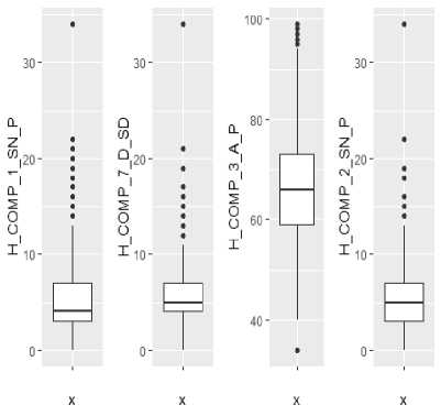
Fig.1. Boxplot for Outlier Detection

• 2)    Variable Selection

In this research, Logistic regression is used to calculate the importance of the variable. We build a regression model using our all the attributes. Applying the ‘summary()’ function to a regression model, we get the description of the features and their relationship with the target variable through the significance. The variable selection results have been displayed in figure 2. Table 1 describes all the significant attributes.

• 3)    Outlier Detection Methods

Outliers are anomalies which are dissimilar from rest of data values. HCAHPS data set after spread involves 38 different important variables. Box plot can be built on each of the variables to detect the outliers. To represent our outlier detection method, we construct a box plot for a few of the variables. Boxplots show us outliers in our data. In all the below series of boxplot the dots represent the outliers. The outliers are valid because each row in our data represent a hospital and removing the outliers will remove a complete row which would cause exclusion one of more hospitals. Thus to avoid the removal of hospitals from the dataset the outliers would exist. Figure 1     represents    the    box plot    for the variables,H_COMP_1_SN_P,H_COMP_7_D_SD_,H_C OMP_3_A_P and H_COMP_2_SN_P.

Table 1. Variables with the most significant P-values

Variable	Description
H_COMP_1_SN_P	How frequently did nurses communicate well with patients? Nurses sometimes or never communicated
H_COMP_3_A_P	How frequently did patients receive help swiftly from hospital staff? Patients always received help when they wanted
H_COMP_7_D_SD	Patients who "Disagreed" or "Strongly Disagreed" that they understood their care when they left the hospital
H_COMP_5_LINEAR_SCORE	It is the linear mean score for communication about medicines
H_COMP_7_LINEAR_SCORE	It is the linear mean score for care transition

		Call: train_data)
glm (formula = myformi	ila, family = binomial, data =
Min	Deviance IQ      Median               3Q	Residuals: Max
-2.9739       -0.0501	9.0661          0.2650	3.1916
Coefficients: (7	not defined because of singularities)
(Intercept)	Estimate Std. Error z value Pr(>|z|) -7.183e+92   2.842eW   - 9.925     9.9798
H CLEAN HSP A P	6.854e+90   2.842e+92     9.924	0.9898
H_CLEAN_HSP_SN_P	6.773e+00   2.842e+92     0.924	0.9810
H_CLEAN_HSP_U_P	6.896e+90   2.842e+92     0.024	0.9899
HCOMPIAP	5.239e-02   5.224e-02     1.003	0.3159
H COMP 1 SN P	-4.465e-01   9.488e-02   -4.796 2.	526-06 ***
HCOMPIUP	NA            NA        NA	NA
H_CDMP_2_A_P	1.494e-92 4.959e-02     0.302	0.7628
H_C0HP_2_SN_P	-1.668e-01 8.859e-02   -1.883	0.0597 .
H COMP 2 и P	NA            NA        NA	NA
H COHP 3 A P	-7.530e-02   3.169e-92   -2.376	0.0175 *
H_C0HP_3_SN_P	-9.521e-92   5.353e-02   -1.779	0.0753 .
H_C0MP_3_U_P	NA            NA        NA	NA
H COHP 5 A P	-4.497e-02   3.312e-02   -1.358	0.1745
H COMP 5 SN P	4.315e-03   4.069e-02     0.106	0.9155
H_COMP_5_U_P	NA            NA        NA	NA
h_comp_6_n_p	-3.584e-92   4.131e-92   -0.868	0.3856
h "comp *6 y"p	NA            NA        NA	NA
H COMP 7 A	-1.llle-92 3.426e-02   -0.324	9.7457
H_C0HP_7_D_SD	-3.997e-91   9.154e-92   -4.366 1.	26e-05 ***
H_C0MP_7_SA	NA            NA        NA	NA
H_QUIET_HSP_A_P	4.399e-92   2.479e-02     1.745	0.0811 .
H QUIET HSP SN P	2.725e-92   4.638e-92     0.588	9.5568
H_QUIET_HSP_U_P	NA            NA        NA	NA
H_CLEAN_LINEAR_SCORE	-1.810e-01    9.736e-02    -1.859	0.9631 .
H_COMP_1_LINEAR_SCORE	-1.1876-01     2.1016-01     -0.565	0.5720
H COMP 2 LINEAR SCORE	1.7406-01    1.566e-01       1.111	0.2666
H COMP 3 LINEAR SCORE	4.895e-02    1.199e-01       9.445	0.6562

h_comp_s_l™ear_sccre	2.483e-01	9.694e-02	2.562	0.0104 *
H_CCHP_6_LMAR_SCORE ■	-3.2756-02	9.9216-02	-0.330	0.7414
H COMP 7 LINEAR SCORE	3.670e-01	1.612e-01	1.177	0.0228 *
H_QUIET_LINEAR_SCORE	1.4556-82	7.8226-02	0.186	0.8524
H_CLEAM_5TAR_RATIMG	5.7016-01	3.174e-01	1.796	0.0724 .
H_COMP_1_STAR_RAT™	2.2606-81	3.468e-01	0.652	0.5147
H COMP 2 STAR RATINE	-3.0866-81	3.3336-01	-0.926	0.3546
H_C0MP_3_5TAR_RATIM3	-6.3096-03	2.9696-01	-0.021	0.9830
H_COMP_5_5TAR_RATING	-1.6016-01	3.2076-01	-0.499	0.6175
H_C0MP_6_5TAR_RAT™	9.3916-02	3.2146-01	0.292	0.7702
H COMP 7 STAR RATINO	5.7966-02	3.4966-01	0.166	0.3683
H_QUIET_STAR_RAn№	3.0886-03	2.8766-01	0.011	0.9914
Signif. codes: 9 111	" 0.001 '“' 0.01 "		0.05 V	0.1 1 1 1
(Dispersion parameter	for binomial family		taken	to be 1)
Null deviance	: 3167.4	on 2397	degrees	of freedom
Residual deviance:	929.5 AIC:	on 2365	degrees	of freedom 995.5

Number of Fisher Scoring iterations: 18

Fig.2. Variable Selection

• IV.    P redictive A nalysis

• A.    Logistic Regression

The goal of the model is to classify the hospital recommendation as ‘yes’ or ‘no.’ Initially, the data is partitioned into the training data, for model training and test data, for testing the model after training to check the accuracy of the model. General linear model (glm) is used to build the Regression model on the training data using below formula. As seen in variable selection section method when logistic regression model is built, considering all the possible attributes, the model gives an accuracy of 90.24 %. To perform predictive analysis, we are building a logistic regression model using only the significant variable identified previously. Equation (1) represents the formula used for logistic regression.

my formula =      ~+HCOMP1 SNP +

HCOMP7DSD + HCOMP3AP +HCOMP5LINEARSCORE + HCOMP7LINEARSCORE

The summary of the model (figure 3) gives the estimates, standard error, z statistics and p-value for the beta coefficients of the regression model and a significance level of the independent variable. In the output, the estimate for H_COMP_1_SN_P indicates that if H_COMP_1_SN_P increases by 1 unit log odds of target decrease by 0.53504, whereas the estimates for H_COMP_3_A_P indicates that if H_COMP_3_A_P increases by 1 unit log odds of target increases by 0.01947. This similarly applies to all the attributes. In the output referring figure 3, the AIC stands for Akaike Information Criterion. It is generally used for comparing models. The model with lower AIC is better. Since we have only one model comparison is not possible.

Call: glm(formula = myformula, family = binomial, data = train_data)

Deviance                             Residuals:

Min              IQ Median              3Q            Max

-3.00825         0.00000         0.08235         0.29421         2.79978

Coefficients:

Estimate Std. Error z value Pr(>|z|)

(Intercept)	-55.47904	6.45474	-8.595	< 2e-16	***
H_COMP_1_SN_P	-0.53504	0.06138	-8.717	< 2e-16	***
H_C0MP_7_D_SD	-6.43559	6.07135	-6.165	1.03e-09	***

H_C0MP_3_A_P                   0.01947      0.01429     1.363      0.173

H_COMP_5_LINEAR_SCORE     0.21229       0.03941     5.387 7.15e-08 ***

H_COMP_7_LINEAR_SCORE     0.53904       0.67399     7.286 3.20e-13 ***

Signif. codes: 6 '***' 6.061        0.61       0.05 ‘6.1 1 ' 1

(Dispersion parameter   for binomial   family   taken   to   be 1)

Null deviance:  3167.44 on  2397    degrees  of  freedom

Residual deviance:     980.62 on 2392 degrees of freedom

AIC:                                 992.62

Number of Fisher Scoring iterations: 9

Fig.3. Logistic Regression Output

The logistics equation for the model is represented in the equation (2) below:

RCMND = exp(-55․47904 + (-0․53504)․ HCOMP 1 SNP

+ (-0.43559). HCOMP 7 DSD

+ 0.01947. HCOMP 3 AP )

+ 0.21229. HCOMP 5 LINEARSCORE

+ 0.53904. HCOMP 7 LINEARSCORE

/ [1

+ exp(-55․47904

+ (-0․53504)․ HCOMP 1 SNP

+ (-0.43559). HCOMP 7 DSD

+ 0.01947. HCOMP 3 AP )

+ 0.21229. HCOMP 5 LINEARSCORE

+ 0.53904. HCOMP 7 LINEARSCORE ]

The bottom half of the output includes the Null deviance and Residual Deviance. Here the Null Deviance represents how well the model performs using only in the intercept, and the Residual Deviance represents how well the model performs using with the intercept and our provided input, the bigger the difference between both the better prediction model performance.

Fig.4. Rpart Decision Tree

• B.    Rpart

Rpart package is used for building the decision tree. In rpart attributes at top level have higher significance. Rpart also has defaults for the fitting function that may stop splitting “early thereby reducing the size of the tree. Parameters like minsplit and minbucket can be used to reduce the size of a large tree. The below-given figure 5 represents the decision tree generated using rpart. Figure 4, decision tree is built only on the attributes selected using the variable selection method. As it can be seen compared to ctree, rpart tree provides exact yes or no value to the target variable instead of indicating the probability of each for the target variable.

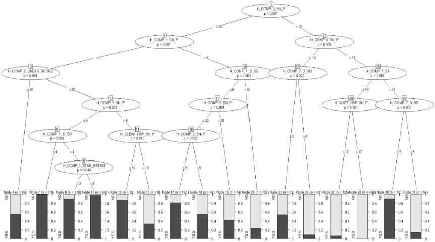
Fig.5. CTree Decision Tree

• C.    Ctree

A decision tree model is built on the preprocessed training dataset using the party package and then evaluated based on the percentage of misclassification on the test data set. Figure 6 represents a binomial tree with 31 nodes. The tree starts at the top and goes downwards. The most significant variable that helps in identifying the target is always at the top. Here H_COMP_3_SN_P is the most crucial variable in classifying the hospital recommendation as yes or no. For each record the model does prediction, it starts with the value of H_COMP_3_SN_P in that record and then continues moving downward till it reaches the leaf node. Each leaf node provides a probability for yes and no representing the probability with which it recommends the hospital and probability with which it does not.

• V.    R esults

This section covers the performance evaluation of all the three models described above. This performance evaluation is carried out using the test data as input.

• A.    Performance Evaluation of the Logistic Regression Model

The assessment of the model is done by running the model against the test data and then comparing the predicted value with the actual value. Performance measure technique like confusion matrix and ROC curve along with Area under the curve are used to evaluate the model. The confusion matrix generated using the test data is represented in figure 6.

Actual

Predicted NO YES

NO 745 85

YES 149 1420

Fig.6. Confusion Matrix for Logistic Regression

From figure 6, the table gives information about the following.

Correct classification: 745 hospitals that are not recommended and the model predicted no for them (True Negative) 1420 hospitals that are recommended and the model predicted yes for them (True Positive)

Misclassification:   149 hospitals that are not recommended but the model predicted yes (False Positive) 85 hospitals that are recommended, but the model predicted no (False Negative)

• •    Sensitivity = TP/ (TP+FN) 1420/(1420+85)= 0.943

• •    Specificity = TN/(FP+TN) 745/(149+745)= 0.833

The accuracy percentage of the model is 90.24%, and the misclassification error percentage of the model is 9.76%.

The ROC curve and Area under Curve (AUC)

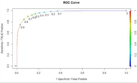
Fig.7. ROC Curve and AUC for Logistic regression

A perfect model has a sensitivity of 1 and a (1 - specificity) of 1. The model performance increases as it approaches closer to this point The above Roc curve build on our logistic regression model records the maximum sensitivity of approximately 0.9, indicating the performance of the curve is good. Based on the curve a threshold can be selected that correctly labels 90 percent of true positive rate with a small false positive rate. Parul Pandey in her article “A Guide to Machine Learning in R for Beginners: Logistic Regression” mentioned that one should select the threshold for the trade-off one wants to make between high specificity and high sensitivity [20]. Each point on the curve represents the ratio between the true positive, i.e. the percentage of hospital recommended yes, and false positive, i.e. the percentage of hospital falsely recommended yes. In the curve, the abline represents that without any model if we predict yes for all the hospital, we will be right 62 percent (total number of yes in the dataset). It acts as a benchmark, curves that lie above the line are better. Another performance metric is AUC i.e. Area under Curve. The value the of AUC ranges from 0 to 1, the closer the value of AUC is to one the better the model. The ROC curve represented in figure 7 has an AUC value of 0.96 thus proving the efficiency of the model.

• B.    Performance Evaluation of Rpart Model

The confusion matrix generated with the help of test data is shown below:

Actual Predicted NO YES NO 735 89 YES 150 1413

• Fig.8. Confusion Matrix for Rpart

From figure 8, the table gives the below information:

Correct classification: 735 hospitals that are not recommended and the model predicted no for them (True Negative) 1413 hospitals that are recommended and the model predicted yes for them (True Positive).

Misclassification: 150 hospitals that are not recommended but the model predicted yes (False Positive) 89 hospitals that are recommended but the model predicted no (False Negative).

• •    Sensitivity  = TP/(TP+FN)  =1413/(1413+89)=

0.940

• •    Specificity = TN/(FP+TN) = 735/(150+735)=

0.830

The accuracy percentage of the model is 89.98% and the misclassification error percentage of the model is 10.02%.

ROC and Area under the Curve

Figure 9 represents the ROC curve for rpart model

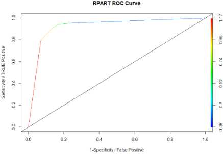
Fig.9. ROC Curve and AUC for Rpart

• C. Perfromance Evaluation of ctree Model

The confusion matrix for ctree is shown below:

Actual Predicted NO YES

NO 739 96 YES 146 1406

Fig.10. Confusion Matrix for CTree

From figure 10, The table gives the below information:

Correct classification: 739 hospitals that are not recommended and the model predicted no for them (True Negative) 1406 hospitals that are recommended and the model predicted yes for them (True Positive).

Misclassification:   146 hospitals that are not recommended but the model predicted yes (False Positive) 96 hospitals that are recommended, but the model predicted no (False Negative).

• •    Sensitivity= TP/ (TP+FN) = 1406/(1406+96)=

0.936

• •    Specificity = TN/(FP+TN) = 739/(146+739)=

0.835 10.14%.

The accuracy percentage of the model is 89.86% and the misclassification error percentage of the model is

• VI. C onclusion and F uture S cope

In this approach, we have proposed a supervised data-driven methodology, which aims at recommending hospitals to the beneficiary based on patient satisfaction measures. Patient satisfaction measures are a necessary asset to perform predictive analysis for hospital recommendation. The analysis approach is explicitly designed for HCAHPS standardized survey which aids the research by handling missing values and deriving predictive analysis over the target variable between layers of data. Prediction models such as decision tree and logistic regression are used for discovering knowledge from data. The summary of the model generate, showcase that     the     recommendation     depends     on

H_COMP_1_SN_P,H_COMP_3_A_P,H_COMP_7_D_S D,H_COMP_5_LINEAR_SCORE,H_COMP_7_LINEA R_SCORE. Interpreting the definition of this attributes we can conclude that if in a hospital, patients receive help as soon as they want it and if patients understand their care then the  hospital  will  receive   a good recommendation, as long as their staff has excellent communication skills. This research, apart from the patients, can also support in the decision making for the hospital representatives regarding how to improve the level of patient satisfaction. It can highlight the areas where the patient service rating was not up to the mark and where the quality needs to be improved. Future work should expand the proposed study to other survey formats for increasing potential benefits, which then give rise to enhanced transparency, healthy decision making and higher incentives for the delivery of good quality health care. In addition to it, the paper can be re-implemented with the availability of HCAHPS latest survey to monitor if there is any improvement in the healthcare organization

Acknowledgment

We would like to thank Dr. Vijay Mago who assisted in putting forward this paper and also guided the way how research should be conducted. The valuable feedback provided by Mr. Dillon Small helped in improving the final reports.