Blow-up of the Solution to the Cauchy Problem for the Equation of Small Oscillations of an Absolutely Flexible Homogeneous Rod

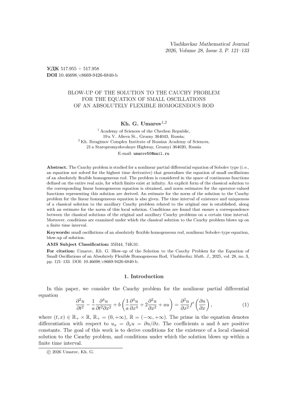
In this paper, we consider the Cauchy problem for the nonlinear partial differential equation

∂ ² u ∂t ²

1 d4 u a ∂t2 ∂x2

/1 d⁴u d ² u \ d^u ‘ ( du\ + b VdX ⁴ +²dX ² + ^au) = dX ² f к dX) ^,

where (t,x) G R + x R , R + = (0, + ro ) , R = ( -от , + от ) . The prime in the equation denotes differentiation with respect to u _x = d _x u = du/dx . The coefficients a and b are positive constants. The goal of this work is to derive conditions for the existence of a local classical solution to the Cauchy problem, and conditions under which the solution blows up within a finite time interval.

Equations of the form (1) belong to the class of pseudohyperb olic equations, as defined in monograph [1, Chapter 2]. In the special case where (f ( • ) = 0) , equation (1) describes small oscillations of an absolutely flexible homogeneous rod [2, Chapter 8, § 43, (8.109)]. It is worth noting that such equations are often referred to as Sobolev-type equations in the literature, since the pioneering work of academician S. L. Sobolev initiated the deep study of partial differential equations that are not resolved with respect to the highest time derivative. Currently, a large number of studies are devoted to various problems involving such equations [3].

The Cauchy problem for equation (1) is considered in the space C[R] [4, Chapter VIII, § 1] of continuous functions g = g(x) for which both limits exist as x ^ ±to, and which are equipped with the norm ||g||c = supxeR |g(x)|. The initial data are given by u|t=0 = ^(x), ut|t=o = ^(x), X € R,

and the sought classical solution u = u(t,x) , (t,x) € R . x R , R ₊ = [0, + ro ) , along with all partial derivatives appearing in equation (1), must for every t belong to C [ R ] with respect to x .

We denote by C ^(k) [ R ] = { g(x) € C [ R ] : g ‘ (x),... ,g ( k (x) € C [ R ] } , for k = 1, 2,... , the subsets of C [ R ] consisting of k -times differentiable functions.

In equation (1), the nonlinearity f(x), x € R, is assumed to be twice continuously differentiable and to satisfy the estimates sup x∈R

I f ⁽ i) (g(x)) | <  f ⁽ⁱ⁾ fsup | g(x)P) ^{1              1}            \xeR        /

i = 0,1   ( V g(x) € C [ R ]),

where | f ⁽⁰⁾ (r) | = | f(r) | and | f ⁽¹⁾ (r) | = | f ‘ (r) | for r € R . are assumed to be non-decreasing functions.

We assume the rod is infinite. This idealization is acceptable [5] if optimal damping devices are placed at the ends of the rod, i.e., the boundary constraints are such that incident perturbations are not reflected.

The investigation of the Cauchy problem (1), (2) will be carried out according to the following plan:

• 1)    We verify that the formulation of the Cauchy problem (1), (2) is correct and that a local-in-time classical solution exists. For this purpose, we first solve the corresponding linear homogeneous equation of type (1). We note that the Cauchy problem for linear Sobolev-type equations with constant coefficients is studied in detail in the fundamental monograph [1], where energy estimates and solvability theorems are obtained in various weighted Sobolev spaces. However, since we are dealing with the nonlinear equation (1), we employ a different approach to derive the solution of the corresponding linear equation and obtain the necessary estimates of auxiliary operator-valued functions. It is also worth mentioning, as pointed out in [6], that adding (or omitting) lower-order terms in an equation not resolved with respect to the highest derivative can significantly affect the solvability of the Cauchy problem.

• 2)    We introduce the auxiliary Cauchy problem

v tt - a — 1 v ttxx + b (a ^-1 v xxxx + 2v xx + av) = d ^ f (v),                  (4)

with initial conditions v|t=o = ^‘(x), vt|t=o = /(x), x € R.

For the Cauchy problem (4), (5), we find a time interval [0, ti] during which a unique classical solution exists, and we estimate its norm in C [ R ] .

• 3)    We establish the connection between the classical solutions u = u(t,x) and v = v(t,x) of equations (1) and (4), respectively, on the interval [0, ti].

• 4)    In the final main section of the paper, we derive sufficient conditions for the blow-up of the classical solution to the Cauchy problem (1), (2) in finite time.

2.    The Cauchy Problem for the Linear Homogeneous Equation

For the reader’s convenience, we also refer to a related article [7].

Let us consider the linear homogeneous equation corresponding to (1):

^u tt

a 1 u ttxx + b (a

U xxxx + 2u xx + au^ — 0.

We introduce a new unknown function:

w(t, x) = u(t, x) - a ^-i u _xx (t, x),

assuming that the partial derivatives u _xx and u _txx are continuous for t G R ₊ . Under the assumption that the initial functions ^(x) , ^(x) belong to C ⁽²⁾ [ R ] , we can uniquely define the initial values of w(t, x) as:

w | t =o = Wo (x) = ^(x) — a ^"(x), W t l t =o = w i (x) = ^(x) — a ⁱ ^"(x).

Using the fact that the positive real axis belongs to the resolvent set of the differential operator d X , we express the solution u(t,x) of equation (6) via the new function w(t,x) as:

u(t, x) = ^1 — a ⁱ dx)

ⁱ w(t,x) = ^a J e ^{l s l}^ a w(t,x + s) ds.

-∞

Here, I denotes the identity operator.

As a result of substitution (8), we obtain the integro-differential equation equivalent to (6):

w tt = (A 2 + Ai )w,

with operator coefficients defined by:

Ai = — 4a ² b(aI - d x ) ^-1 , D(A i ) = C [ R ]; A2 = bd ² _x + 3ab, D(A 2 ) = C ⁽²⁾ [ R ].

In the space C [ R ] , the operator bd 2 generates a strongly continuous cosine operator function C ( t ; bd 2 ) , т G R , which is represented on elements g(x) G C [ R ] as [8, § 1.5]:

C(t; bdx)g(x) = 2 [g(x + т^ + g(x - TVb)], and satisfies the norm estimate:

||C (t; ьд ²   <  1, t G R₊.

The perturbed operator A2 = bd X + 3ab generates a strongly continuous cosine operator function C ( t ; A2) , т G R , which for any g(x) G C [ R ] has the representation [8, §8.2]:

τ

C ( t ; A ₂ )g(x) = C ( t ; bd 2 )g(x) + т V 3ab J 0

I _i (у/3аЬ(т ²

V t ² — s ²

s ² ) )

---— C(s; bd 2 ) g(x) ds,

where Ii( ^ ) is the modified Bessel function of the first kind. The corresponding norm estimate is:

||C(t; A ₂ ) | C cosh (t V 3ab), t G R +.

The bounded operator Ai = - 4a ² b(aI — d X ) ^-1 , with | A1 | C 4ab , generates a cosine operator function C ( t ; Ai) continuous in the uniform operator topology, which has the representation [8, § 1.4, § 4.2]:

“ _T 2 n

C ( t ; Ai)g(x) = £      A n g(x) ( V g(x) G C [ R ]), т G R ,

(2n)! n =0 ^{v 7}

with the estimate:

| C(t; Ai) | C cosh (2t V ab), t G R ₊ .

The operator A = A2 + Ai results from the bounded perturbation of the unbounded operator A2 by Ai . Since bounded perturbations preserve the cosine generator property [8, §8.2], A generates a strongly continuous cosine operator function C (т; A) , т G R , which satisfies the representation for g(x) G C [ R ] :

i

_T 2

C(т; A)g(x) = C(т; A2)g(x) + у j j (тV1 — s2, Ai) AiC(ts; A2)g(x) ds, where

i j1(т,A1 )g(x) = П J V1 — r2 C(тг; Ai)g(x) dr.

For t G R . , the following norm estimates hold:

ji (tAi^l ^C —1= ^I 1 (2^t V a^b)^, t ab

\\C (t; A) || C cosh (t V 3ab) + ^ cosh (2t V 7ab) =: h _i (t).                 (10)

Associated with the cosine function C (т; A) is the sine operator function [8, § 1.4]:

τ

S (т; A)g(x) = У C (s; A)g(x) ds, g(x) G C [ R ], 0

and the linear manifold

Ci[ R ] = { g(x) g C[ R ] : C(т; A)g(x) G C ⁱ ( R ,C[ R ]) } .

That is, Ci[ R ] C C [ R ] consists of those functions for which C (т; A)g(x) is continuously differentiable in т . Clearly, D (A) = C ⁽²⁾ [ R ] C C _i [ R ] .

Using estimate (10), we obtain sinh (tV3ab) sinh (2t^7ab) z 4                          z 4

\ S (t; A) | C---- +-5=U =: h2(t),  t G R ₊ .          (11)

V 3ab          4y7ab

Equation (9) can be rewritten in the space C [ R ] as an abstract second-order differential equation:

W tt = AW, t G R ₊ ,                            (12)

where W = W(t) : t H w (t,x) is the desired vector-valued function defined for t G R ₊ with values in C [ R ] .

For equation (12), we consider the abstract Cauchy problem with initial conditions:

W | t =o = Wo, W t | t =o = W i ,                           (13)

where Wo = wo(x) , Wi = w i (x) are elements of the space C [ R ] .

The Cauchy problem (12), (13) is uniformly well-posed [8, § 1.4] only when the operator A is the generator of a strongly continuous cosine operator function C(t; A) . In this case, the solution to the abstract Cauchy problem is given by the formula W(t) = C(t; A)W o + S(t; A)W _i for any Wo G D (A) and W _i G C _i [ R ] [8, § 1.4].

Now, by applying the inverse transformation (8) and taking into account the commutativity of the resolvent (I — a ^{- i} d‘ X ) ^{- i} with the cosine operator function C(t; A) , we obtain the solution to the Cauchy problem (6), (2):

u(t,x)= C(t; A)^(x) + S(t; A)^(x), t G R ₊ .                    (14)

Thus, we have

Lemma 1. Let the initial functions ^(x), ^(x) belong to C ⁽⁴⁾ [ R ] . Then the Cauchy problem (6), (2) is uniformly well-posed, its classical solution is given by formula (14), and the following estimate holds:

sup |u(t, x)| < h1(t) sup |^(x)| + h2(t) sup |^(x)|, x∈R                 x∈R               x∈R where the functions hi(t) and h?(t) are defined by inequalities (10) and (11).

Remark 1. The classical solution W(t) of the abstract Cauchy problem (12), (13) belongs to C ⁽²⁾ ( R ₊ ,C[ R ]) and satisfies AW(t) G C ( R +,C[ R ]) ; therefore, the solution u(t,x) of equation (6) belongs to C ^2,4 ( R ₊ , R ) .

• 3.    Local Solution of the Cauchy Problem for the Nonlinear Equation (4)

Equation (4) is obtained from equation (1) by differentiating both sides with respect to x and making the substitution u _x = v (the left-hand sides of these equations coincide).

Applying the operator (I — a ^{- i} d X ) ^{- i} to both sides of equation (4), we obtain an equivalent integro-differential equation, which can be written in the space C [ R ] as the following abstract semilinear equation:

V tt = AV + F (V),                              (15)

where V = V(t) : t H v(t,x) is the sought vector-valued function, and the operator A is as in equation (12).

The nonlinear operator F ( • ) in equation (15) is defined by

F(g) = a [a(aI — dX)-i — I] f (g), where f(•) is the Nemytskii (superposition) operator: f (д') = f(g(x)), g(x) G C[R], and satisfies the norm estimate:

||F (g)|| c <  2a | f ( | g | c ) | , g G C [ R ].

For equation (15), we consider the abstract Cauchy problem with initial conditions:

V | t =0 = Vo,    V t | t =0 = V1,                                (17)

where Vo = ^ ' (x) , V1 = f ' (x) are elements of C [ R ] .

The continuous differentiability of the superposition operator in the space of continuous functions, and the boundedness of the linear operator (al — d X ) ^-i , imply the Frechet differentiability of F ( • ) in C [ R ] . Therefore, there exists an interval [0, to) on which the abstract Cauchy problem (15), (17) has [9, §3] a unique classical solution V = V(t) that satisfies the abstract integral equation

t

• V(t) = C(t; A) Vo + S(t; A) Vi + J S(t — т ; A)F(V ( t )) dT,             (18)

for any V0 € D (A) and V _i G C _i [ R ] .

From the integral equation (18), using the estimates (10), (11), (16), and (3), we derive the integral inequality

t

I V(t) | c C hi(t)||Vo|| c + h2(t)||Vi lie + 2aj h ₂ (t — т ) I f ( N V ( t ) ( c ) | dT, 0

^where IIVoll e     ^sUP x . . |^ ' ^(x)h IIVill e =SUP x _{e R} ^'(x)| .

Let ki = max (hi(t)|Vo|e + h2(t)|Vi|e),   k2 = 2a max h2(t), te[o,to]                                                                      te[o,to]

and increasing the right-hand side of the integral inequality, we have

t

I V(t) | c C ki + k2 У | f( N V(T ) | c ) | dT.                         (19)

o

From inequality (19), we obtain [10, Chapter 1, § 1.4] an estimate for the norm of the classical solution of the abstract Cauchy problem (15), (17) in the space C [ R ] on the interval [0,ti] :

|V(t)le c G-i (G(ki) + k2t) =: h3(t), where G(t) = ft |fdS)| for T,t > 0, G-i(•) is the inverse function to G(-), and the interval [0, ti] C [0, to) is determined by those t for which G(ki) + k2t lies in the domain of definition of G-iG).

Thus, we have

Lemma 2. Let the function f ( • ) satisfy condition (3) , and let the initial functions ^(x) and ^(x) belong to C [ R ] together with their derivatives up to order five inclusive. Then on the interval [0,ti] , there exists a unique classical solution v = v(t, x) to the Cauchy problem (4) , (5) , for which the following estimate holds:

sup | v(t,x) | = sup | u _X (t,x) | C h3(t), t G [0,t _i ].                       (20)

x ∈ R            x ∈ R

4.    Connection Between Solutions of Equations (1) and (4)

Assume that the classical solution v = v(t,x) = u x (t,x) of the auxiliary Cauchy problem (4), (5), along with its partial derivatives v _XX (t, x) , v _ttxx (t,x) , v _xxxx (t, x) , v _xx (t,x) , and the functions v X (t, x) • f ‘ (v(t,x)) and v _xx (t,x) • f ‘‘ (v(t,x)) , for all values of the time variable t G [0, ti] , belong (with respect to x ) to the intersection of the space C [ R ] with the space L1( R ) of absolutely integrable functions, i. e., J - + ^ \ g(x) \ dx <  от . All these requirements are satisfied if on the time interval t G [0, ti] the following conditions hold:

u _x , u _ttx , u _ttxxx , u _xxxxx , u _xxx , u _xx

f ‘ (u x ),u xxx • f ‘‘ (и х ) G C [ R ] П Li( R ).

Note that from the fact that g(x) G C [ R ] П Li( R ) , i.e., the integral J j + ^ \ g(x) \ dx <  от converges and the limits lim _x ^±_№ g(x) exist, it follows [11, Ch. 2, §29.1] that these limits are equal to zero: lim _x ^±_№ g(x) = 0 .

Lemma 3. The existence of a local classical solution v = v(t, x), t G [0, ti], to the Cauchy problem (4), (5) implies the existence of the corresponding solution и = u(t, x)

= lim x0→-∞

x

/ v(t,s)

ds

x v (t, s) ds

-∞ to the Cauchy problem (1), (2) on the same time interval [0, ti], provided conditions (21) and the following limiting relations hold:

Utt,UtXx_X,Uxxx_X,Ux_X,u ^ 0 as x 4-от , t G [0,ti].

<1 Let v = v(t,x) = u _x (t, x) , t G [0,ti] , be a classical solution of equation (4). Then using the limiting relations (23), we obtain:

x

J d S f (v(t,s)) ds

-∞

x

У [u 2 s (t, s)f ‘ (U s (t, s)) + U sss (t, s)f ‘‘ (u _s (t, s)) ] ds

-∞

= U xx (t,x)f ‘ (U x (t,x)) - lim U xx (t,x o )f ‘ (U x (t,x o )) = U xx (t,x)f ‘ (U x (t,x)). x 0 →-∞

Now, substituting expression (22) into equation (1), we obtain an identity on the interval [0, ti] , which implies that the function (22) is a solution of equation (1). >

5.    Blow-Up of the Classical Solution to the Cauchy Problem (1), (2)

In the subsequent analysis, it is assumed that the classical solution и = u(t, x) , (t, x) G [0, ti] x R , of the Cauchy problem (1), (2), together with the partial derivatives appearing in equation (1), belongs to the intersection of the space C [ R ] and the space L2( R ) of square-integrable functions. All these requirements are satisfied if, on the time interval t G [0,ti] , the following conditions hold:

d tn d xm u(t, x) G C [ R ] П L ₂ ( R ), n + m <  4, n = 0,1, 2, m = 0,1, 2, 3,4.        (24)

Such a solution will be called a classical solution of the Cauchy problem (1), (2) in the space L2( R ) .

Note that from conditions (24) it follows that the following limiting relations hold:

lim   dtd™u(t, x) = 0,    n + m C 4, n = 0,1, 2, m = 0,1, 2, 3,4, t G [0, ti].     (25)

Recall that the inner product and norm in L2(R) are defined by the formulas:

+ ∞                 + ∞

(^^ У KM^x) dx, IMl2 = У M^{x)| 2} dx.

-∞

-∞

On the time interval t G [0, ti] for which a classical solution u = u(t, x) of the Cauchy problem (1), (2) exists, we introduce the functional:

+ ∞

y(t) = (u,u) + a ^-1 (u x ,u x )= У (u ² + a

-∞

1u X ) dx, t G [0, t 1 ].

Applying the derivative to the functional y(t) gives: y ‘ (t) = 2 ((u, ut) + a - 1 (u x ,u tx )) , the Cauchy-Schwarz inequality: | (^,^) | C IMI2 IMh> and, denoting

z(t) = (u t , u t ) + a 1 (u tx ,u tx ) = У (u2 + a

-∞

1u2_x) dx, t G [0, t 1 ],

which is another functional related to equation (1), we obtain the auxiliary estimate:

⁽y ‘ ^(t))2 ^C 4y^(t)z(t)-

We now seek sufficient conditions for the blow-up of the solution of the Cauchy problem (1), (2), meaning the appearance of a discontinuity of the second kind for the functional y(t) on some interval [0,t2] C [0,ti] , which is chosen such that y(t) >  0 and y ‘ (t) ^ 0 hold, resulting from the initial conditions y(0) > 0 and y ‘ (0) > 0 .

Theorem. Suppose the conditions of Lemmas 2 and 3 are satisfied and that the initial functions ^(x) and ^(x) and the nonlinearity f ( • ) meet the following requirements:

Ь^2 + a

11И12 > 0, (^,^) + a K,/) >  0,

2by 112 + IK + a

x

^H(2 + (fW ,^) >a "W' H2 + ab|Ml2,

F (x) = у f (s) ds >  0 ( V x G R);   F (u x ) G L i (R),

11^12 + a

1IIK + a ^-1

^Ь1К12 + ^abH^H2 + ² У F(^ ' ^(x))dx >  ²b ^I ^ ‘ ^I 2 ,

-∞

((^H a KK) ² > (IMI2 + a

11И2)

2b( x I b—-

a + 2b) + 2a + кз

ak3

(м2 + a M112)+Eo),

then the classical solution u = u(t, x) of the Cauchy problem (1), (2) in the space L2(R) blows up in finite time ak3

T ■ C k-1 (IMl2 + a-1|Ml2)-4b , and moreover, the following lower bound holds for the functional:

y(t) = INi + a 1 h u x h 2 >

_ ak 3

1И2 + a -Wll!) - 4b

_- 4b

) ako

where the constants k i and E 0 are determined by the parameters a, b, the initial functions ^(x), ^(x), and the nonlinearity f ( • ) .

<1 Multiply both sides of equation (1) by u = u(t,x) and integrate the resulting equality over x from —от to + ot . Then, integrating by parts and using the limiting relations (25), we obtain

(u tt ,u)+ a 1 (u ttx ,u x ) + a ¹ b(u xx ,U xx ) — 2b(u x ,U x ) + ab(u,u) — (f ‘ (u x )u xx ,u) = 0. (27)

Using the representations

(u tt ,u) = -( u t ,u) — (u t ,u t ) = - -2 ||u||2 dt                     2 dt

—

| u t | 2,

d                          1 d ²

(u ttx ,u x ) = — (u tx ,u x ) — (u tx ,u tx ) = ^ d! IK | 2

—

llutx ^h 2 ,

and

(u tt ,u) + a 1 (u ttx ,u x ) = 2 y " (t) — z(t),

from (27) we derive the equality

y ” (t) + 2a ¹ b || u_xx || 22, + 2ab h u h 2 — 2(f ‘ (u x )u xx ,u) = 4b | u x | 2 + 2z(t).

From equation (28) we find the value at zero of the second derivative of the functional y(t) , and require the following condition to hold:

2b|Kll2 + KII2 + a-¹HII2 + (f‘&>", ^) — a-¹b h ^ I 2 — abIMI2 >  0,

then on some interval [0, t3] C [0, t2] the inequality y ‘‘ (t) ^ 0 will be satisfied.

Applying inequalities (3) and (20), we estimate the fourth term on the left-hand side of equality (28):

— 2(f (u _x )u _xx

u) C 2 У | f ‘ (u x ) || u xx || u | dx C 2

-∞

f ‘ [ sup | ux | I x ∈ R

(using the Cauchy–Schwarz inequality)

( | u xx | , | u | )

C 2|f ‘(h3 (t))\luxx ||2 |u|2 С кз (||uxx||2 + |u|2) , where кз = maxte[o,t1] \f‘(h3(t))\.

Taking into account the sequence of inequalities (29), we increase the left-hand side of equality (28) while simultaneously decreasing the right-hand side:

y ‘‘ (t) + (2a ^-1 b + k3) | u xx | 2 + (2ab + k3) | u | 2 >  2z(t),   t e [0,t3].           (30)

Multiply both sides of equation (1) by u t = u t (t,x) and integrate the resulting equality over x from —от to + ot . Then, integrating by parts, we have

(u tt ,u t ) + a^-1(u ttx ,u tx ) + a^-1b(u xx ,u txx ) — 2b(u x ,u tx ) + ab(u,u t ) + (f (u x ),u tx ) = 0. (31)

Denote by F ( • ) the function determined by the nonlinearity of equation (1):

x

F (x) = I

^{f (s)} ds,

and assuming F(u _x ) G Li(R) , t G [0,t3] , from equality (31) we obtain

1 d

2 dtE(t)=0, where E(t) is the functional associated with equation (1):

^E(t) = H u t H 2 + a 1 ^ u tx ^ 2 + a 1 ^b ^ ^u xx ^ 2

- ^2b \\ u x \\ 2 + abllull! +²

+ ∞

У F(u x ) dx.

-∞

From equality (32) it follows that E(t) does not depend on time, and therefore the equality holds

E(t) = E(0) = Eo,                                (33)

where the constant E 0 is defined by the formula

Eo = Ml! + a^-1Hll! + a ^{- 1} b \ ^ \ 2

^{— 2b} \ ^ ' \ 2 + abll^ Il2 +²

+ ∞

У F(^ (x)) dx.

-∞

Let Eo ^ 0 , and let the nonlinearity of equation (1) satisfy the condition

x

F (x) = I

f (s) ds ^ 0

( V x G R).

Note that the set of functions f ( • ) satisfying condition (34) is not empty. Indeed, for example, the functions f (x) = x ²ⁿ⁺¹ , where n >  0 , satisfy condition (34).

Rewrite equality (33) as

+ ∞

z^(t) + a 1 b \ u xx \ 2 + ^(a + ^2)b \ u \ 2 + ²

У F(их) dx = Eo + 2by(t).

-∞

Decreasing the left-hand side of equality (35), we derive the estimate

\ u xx \ 2 <  ab 1 (E o + 2by(t) — z(t)).                           (36)

Using inequality (26), we decrease the right-hand side, and applying inequalities (36) and I|u|l 2 ^ y(t) , we increase the left-hand side of inequality (30). Then we obtain the differential inequality

y(t)y " (t) — k 4 (y'(t)) 2 + k 5 y 2 (t) + k 6 y(t) >  0, t G [0, t ₃ ], (37)

where the coefficients are computed by the formulas ak3

k4 -1 + 1T

k5 — 2b(a + 2) + (2a + 1)кз,

k6 — (2 + ak3 ) Eo,

and we note that k4 > 1 and 5 — 1 — 1—4^4 — 2(1 + 023) > 0. Let the initial conditions hold y‘(0) > (ГЧ<«<“))’ + k y(0)^ ’ — 2 (b2b(a          + 1)k3 (y(0))2 + ЗД0)(

( k4 — 1          (k4 — 1)5    /      (           акз                           / or, substituting the values of y(0) and y'(0),

(fe ♦) + i(/, V/) ) ² >  b ^{2b(a + 2} + (2a +1)k} 3 (|M| 2 + ¹ | _? ‘ И ² ) ² + Eo (m² + ¹ Il l 'll ²' ) . a                      ak3                  a                      a

Then, comparing inequality (37) with an ordinary differential inequality [12, Appendix, § 2, (2.38)], we conclude that for the time t3 of existence of the solution to the Cauchy problem (1), (2), the following upper estimate holds t3 < Tm C

1 k7(y(0)) k ⁴ ■

MlMli+ а-11И12) ^b

where k2 — .     ■ 4 [(y‘(0))2 — k;^

^—У3 (^|₽|2^+а-11И^|г)^-2-[(W’)+«^-1(f',*'))²

—b^{2b(a + 2b}) ^{+ 2a + k}3 (j^j2 + a-¹^|2)²— Eo(_|M|2 + _O-1_M|2) , ak3

and for the functional y(t) — |u|2 + a^-1|uxHi the following lower bound holds

y^(t) >

((y(0))^1-k4 — kyt) k4^-1

(M + а-11И12)" ak³— kit) a⁴³

and, therefore, lim y(t) — +to.

t↑T∞

The author of the article expresses gratitude to the reviewer for careful reading of the article and comments made.