Cauchy fractional derivative

Cauchy's integral formula for derivatives is given by the following relation

F”)   =   ,Fwdw , s £     , n n+1 ,                 7,

^{2 n} i C ( w - s )

It calculates the derivative of order n of an analytic function when n is a nonnegative integer.

Also, it seems to calculate the derivative of fractional order when we write a > 0 instead of n :

Г ( a + 1)   F(w)dw

^F ' ^{) (} s ) = Л^ПгЧ^ • s ⁶ 'nt ^{( C} ) •                  (1)

^{2 n i} _C ( w - s )

However, it is not as simple as it looks. Because the contour integral in the formula (1) is so complicated. Moreover, the function (w - s )a+1 is multi-varied. Hence, the value of the contour integral in (1) is not independent of the choice of closed curve C . Formula (1) is an unpractical one to calculate the fractional derivative of a function. Therefore, it needs a modification. Here, we modify the formula (1). By making some calculations, we return it to the formula

F ^(a ) ( s ) ■ L { ( - x )^a L "¹ { F } } ,                                     (2)

where L is the Laplace transform.

Weyl's fractional derivative is given by the following formula swa (s) ■

( - 1 ) ^a    d^{n J} F ( t ) dt

r ( n - a ) dsⁿ ’ ( t - s )^{a - n + 1}

where s >0, n-1< a < n, n бМ, a >0 [1]. Raina and Koul [1] proved in 1979 that the Laplace transform of the function (-x)a f (x) is equal to atA derivative, in the sense of Weyl, of the Laplace transform of f . This means that the fractional derivative of a function F with the inverse Laplace transform can be calculated by the following formula swa F ( s ) ■ L {(- x )a L"1 { F }}•                                 (4)

In this work, we move the contour integral in the formula (1) to an infinite vertical line, and then we prove the relation (2). Finally, we give some examples.

Laplace Transform and Cauchy's Integral Formula for Derivatives

Let f be a continuous function from [0, +j) to C and satisfy the inequality |f (x)| < Mea for some a, M 6 R. Then, its Laplace transform is defined by the following да

L {f} = Jf (x) e - sxdx, where Re (s) > a and a eR. We denote the Laplace transform of a function f by F (s), i.e.

F ( s ) = J f ( x ) e - sx dx.

For example, the Laplace transform of the function f ( x ) = ( - x ) ^a e^wx is

F ( s ) = -   :— a+1

⁽ w ^- s )

where a > 0, Re ( s ) >  Re ( w ) and Г is the gamma function given by

Г ( z ) = J x z ^{- 1} e ^- x dx .

Laplace transform forms an invertible linear operator. Mellin's inverse formula for Laplace operator is given by the line integral:

c ⁺ i да

■ f (x)" 21/ J F (w) С'"М

c - i да where c is a suitable real constant [2].

Now, we recall Cauchy's integral formula for derivative. Assume that D is a region in the Complex plane C , F is an analytic function in D, s e D, C is a curve satisfying the condition s e int (C) and n e N; then the nth derivative of F is given by the following formula [3]

F ^{( n} ) ( s ) =

n ! F ( w ) dw 2 ni C ( w - s) n + ^r.

Cauchy's Integral Formula for Derivatives on an Infinite Vertical Line

Lemma 1. Assume that F and f are two functions satisfying the condition (5). Then, F is an analytic function in the region Re ( s ) >  a and it is bounded in the region Re ( s ) > c for each c > a . Besides, the improper integral in (5) is uniformly convergent on the region Re ( s ) >  c [2].

Definition 1. If a function F is the Laplace transform of a function, then we state that it is a Laplace type function.

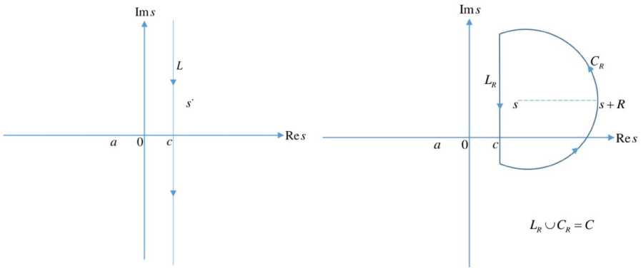
Fig. 1. Infinite vertical line

Fig. 2. Half circle

Lemma 2. Let F be a Laplace type function and n g N. Then, Cauchy's integral formula for derivatives (see (8)) can be written as follows:

F ( " ) ( s ) = ~c-i '^{№ F ( w} ) dw

-ПL(w- ■ )" +r where a < c < Re (s). Note that the integral above is taken on the infinite vertical line L shown in

Figure 1.

Proof. By Cauchy's integral formula for derivatives (8) and by the structure of the curve C shown in the Figure 2, we obtain

F (”)( s ) = n! Fjwdwl n! r F (w) dw   n! r F (w) dw w - s) n'  +          w - s)'''"

’  2 ni J ( _w - s ) ^{n + 1}

By Lemma 1, there exists a positive number M such that |F (w)| < M. Then, we have n! r F (w) dw

^kww - s ) n ^{+ 1}

n!  , |F(w)| |dw Mn! г |      Mn!

" 2 n / w - s i n ^{+ 1} ”2 nR^{n + 1} J w  2 Rⁿ '

C _R                     C _R

The last relation shows that the value of the integral on the half circle C_R vanishes when R ^ +№ .

This ends the proof.

Cauchy Fractional Derivative

Definition 2. Let F be a Laplace type function and a be a positive real number. We denote Cauchy fractional derivative of order a by sCaF (s) and define as the following relation sca f (s)=

Г ( а + 1 ) ^c i ^№ F ( w ) dw ^{2 П} c U w - s ) ^{a + 1} ’

where a < c < Re ( s ) (see Fig. 1).

Remark. Since the function F in the formula (9) is a Laplace type function, then there exists at least one real number a such that F is analytic in the region Re ( w ) >  a . Furthermore, the function

(w - s )a+1 has inf {k g N | ka g N} analytic branches in the region

C \ { w = £ + Um ( s ) | § >  Re ( s ) } .

So, there are inf { k g N | ka g N} values of Cauchy fractional derivative for any function F . And also, one can simply see that these values are independent of the choice of the real number c in the interval ( a , Re ( s )) .

Theorem 1. Let F be a Laplace type function and a be a positive real number. Then the Cauchy fractional derivative sC^F (s) holds the following relation scaF(s) = L{(-x)aL"1 {F}} = s waF(s).

Proof. We begin by writing the definition of the Cauchy fractional derivative:

₅C ^ F ( s ) = — c - i ^№ F ( w ) ^{r( a +} 1 ) dw.

^{s №}     ’  2ni c +^J№ ¹ 4 w - s ) ^{a + 1}

By the formula (6), we obtain c - i№

sC№F(s) = -J F(w)L{(-x)aew} c+i №

4  c +1 №         № dw =---; j F (w) J(-x)a e(w-s)xdx dw.

^{2 Пг} c - i №       к 0                  J

c + i №

№

By using the uniform convergence of the Laplace's improper integral and the boundedness of the function F (see Lemma 1), we can change the order of integration, i.e.

1 да c+i да                                             да sCF(s) = — J J F(w)(-xГ e(w-s)xdwdx = J(-x)“ e 2ni

0 c - г да                                        0

- sx

ч c + 1 да

--- [ F ( w ) e wx dw dx.

2ni J V '

c - 1 да                  У

c + i да

By the inverse Laplace formula (7), the fractional derivative _sC ^ F ( s ) can be written as

CF ( s ) = да ( - x )^a e ^{- sx} L"^x { F } dx = L { ( - x )^a L "¹ { F } } .                  (10)

The formulas (4) and (10) completes the proof.

• Example 1. By using well-known formula

^{L { x} r ^{- 1 }} = IT, ^r >0

we have

5 ca — = L 1(-x)a L~x I - s да

s        I               I s

Г ( г ) L

(~FLT[xa+r-Й _ «Г(а + r) Г(r)   {       } Г( r)sa+r ‘

In a similar way, we can obtain the following

C a ¹    = (-У У Г ^ О + г )

s ^да ( s - a ) r   Г ( r )( s - a )^{a +} r ,

where a g C .

th

A table of some functions'

derivatives is given in the following:

th derivative of some functions

Function, F ( s )

th                           ¹

• — derivative, _sC да - F ( s )

1 arctan

s

s ² + 1

s s 27i

ln s

s

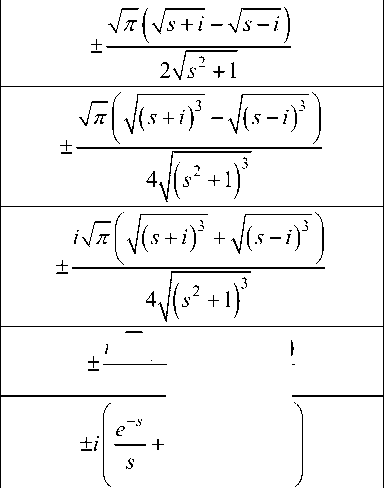
2 s ³²

Пе erfc ( 4s )

2 s ³²

i 4П ( In s + 2ln2 - 2 )

Example 2. We can use the Dirac Delta function, which is a generalized function denoted by 3 ( x )

and defined by the equality

f TO

J -TO

3 ( x - b ) f ( x ) = f ( b ) , to calculate the Cauchy fractional derivative. Let

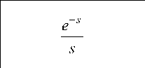
F ( 5 ) = e- b ⁵ , b >0. Then, the inverse Laplace transform of it is 3 ( x - b ) and we have ₅^ “ e ^- b ⁵ = L { ( - x )^a L ¹ { e ^- b ⁵ } } = L { ( - x )^a 3 ( x - b ) } = ( -b ^“ e ^{- bs} . To illustrate,

5 ^ 2 e⁵ = ± ie⁵ .