CFD-based Analysis of Aeroelastic behavior of Supersonic Fins

Published Online February 2011 in MECS

Computational aeroelasticity is one of the most challenging fields for aircraft. For an aircraft in flight, strong interactions can occur between the flexible aircraft structures and the surrounding flow resulting in aeroelastic problems[1, 2]. The emphasis of the study is the discipline of displacement and load of the flexible structure under the unsteady aerodynamic. The coupling of computational fluid dynamics (CFD) and computational structural dynamics (CSD) tools to solve aeroelastic problems has received a strong interest in the recent years[3, 4].

Direct incorporation of a CFD code into a fluidstructure interface solver leads to high computational cost. One solution to this problem is the development of aerodynamic reduced order models (ROMs). Silva first proposed a Volterra kernel ROM approach, which is one of several ROMs currently being used[5]. The Volterrabased ROM approach has been used extensively for solving fluid-structure interaction phenomena including nonlinear computational fluid dynamics using Euler/Navier-Stokes models and linear structural dynamic

Supported by the National natural Science Foundation of China (Grant No.90816008) and Doctoral Fund of Ministry of Education of China(Gant No.20070699054)

solvers[6].

Although a significant amount of research has been conducted in the area of aeroelasticity, most solutions only address to the flutter boundary of aircraft[7], but practice has proved that an aircraft may take place serious aeroelastic phenomenon under the flutter boundary[8]. The focus of present paper is to analyze the flutter boundary and transient loads of a supersonic fin.

Aircraft received a variety of perturbation in flight, such as the vibration of engine, the roll of body or the change of attack, these kinds of perturbation will affect the aeroelastic stability of structure[15]. Then The structure has two parts of movement, the rigidity movement caused by roll of missile body and the response of aeroelasticity, and the rigidity movement affect the elastic response by the append aerodynamic, so the perturbation may reduce the flutter boundary.

• II.    A EROELASTIC ANALYSIS BASED ON CFD/CSD

• A.    Structural Dynamics Equations

In the generalized coordinates, the multi mode system of equations can be expressed in matrix notation as:

Where § is the generalized displacement vector , M is the identity matrix; Q is the generalized buffeting force vector, C and K are respectively the generalized total damping and stiffness matrices[9].

• B.    Coupling Algorithm

An aeroelastic system can be viewed as the coupling of an unsteady aerodynamic system with a structural system. The coupled solution is based on a time-domain partitioned solution process in which the nonlinear partial differential equations modeling the dynamic behavior of both fluid and structure are solved independently with boundary information (aerodynamic loads and structural displacements) being shared alternately. A schematic of the framework is shown in figure 1. The aeroelastic problem is solved using a partitioned approach to couple the CFD and CSD solutions, both solvers are called once per coupled time-step while exchanging data at the interface. A dedicated interface module was developed to enable communication between the flow and the structure at the 3-D wetted surface (fluid-structure interface)[10,11].

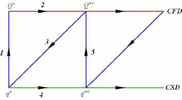
Figure 1. Schematic of the aeroelastic framework

• C.    Fluid-Structure Interpolation(FSI)

FSI is applicable to many engineering fields, and in conventional aerospace engineering applications, is known as aeroelasticity. Numerical methods to simulate FSI have been under development for many years. To perform interpolation of physical quantities between the fluid and the structural grids, the infinite plate spline is included in the aeroelastic framework. The infinite plate spline is a global interpolation approach, and its distribution function is given by[12]:

N w (x, y) = a 0 + a1 x + a 2 y + Z Ki (x, y)Fi i=1

(2) Where:

K ( x , y ) = r²ln r²

2             2             2                    (3)

ri =( x - xi) +(y - y)

The n+3 unknowns ( ^{a 0 , a 1 , a 2 , F} ) are determined from

the n+3 equations:
	■ 0 "		■0	0	0	1	L	1 "	a 0
	0		0	0	0	x 1	L	x N	a 1
	0		0	0	0	y 1	L	y N	a 2
	w 1	=	1	x 1	y 1	0	L	K 1 N	F 1	(4)
	w 2		1	x 2	y 2	K 21	L	K 2 N	F 2
	M		M	M	M	M	L	M	M
	_ W n _		_1	xN	yN	KN 1	L	0	_ F n _

III. F LUTTER PREDICTION BASED ON ROM

• A.    Volterra-Based ROM Approach

At present, the development of CFD-based ROMs is an area of active research at several industry, government, and academic institutions. Development of ROMs based on the Volterra theory is one of several ROM methods currently under development. Reduced-order models based on the Volterra theory have been applied successfully to Euler and Navier-Stokes models of nonlinear unsteady aerodynamic and aeroelastic systems.

The Euler equations can be considered weakly nonlinear and can be accurately represented by a truncated second order Volterra series. Linear response models have often been used to represent nonlinear aerodynamic systems when excited by small perturbations. This is based on the fact that highly nonlinear phenomena have negligible impact on the net effect of various responses under conditions of small perturbation excitations. Generally, the responses can be expressed as[13]:

n y (n) = h0 + Z h (n - k) u (k) + k=0

nn zzh 2(n - k1, n - k 2 )u (k1) u (k 2)

k , = 0 k ₂ = 0

The convolution of the derivative of step response is chosen as a method of choice in building the aerodynamic ROM. Convolution of the derivative of the step response generates a predicted response that is a superposition of the convolution of first-order Volterra kernel, the convolution of the averaged diagonal terms of second-order kernel that are present in the convolution of the pulse response and a convolution of the averaged nondiagonal terms.

n = 0

h ( n ) + 5, h 2 ( n , n )

% ( n ) =.

Г,.                ) _ (6)

h(n ) + 5 h(n , n ) + 2Z h^n,n - k) n -0 k : 1^zv         ')

The step responses Volterra kernels are then used with the Eigensystem Realisation Algorithm (ERA), to generate a linear time-continuous state-space system, then coupled with structure as a Aeroelastic ROM model[14].

An outline of the ROM development process is as follows:

• 1.    Implementation of step response technique into aeroelastic CFD code;

• 2.    Computation of step responses for each mode of an aeroelastic system using the aeroelastic CFD code;

• 3.    Step responses generated in Step 2 are input into the ERA;

• 4.    Evaluation/validation of the state-space models generated in Step 3;

• B.    Flutter Pred ct on of a Superson c F n

0.0002

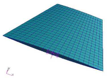
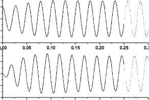
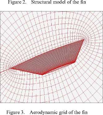
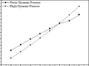
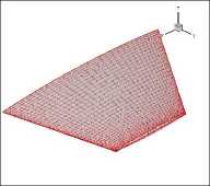
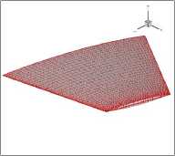
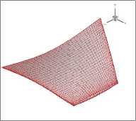
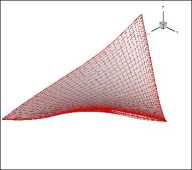
A low-aspect-ratio supersonic fin, as shown in figure 2, is selected as a test case for Flutter Boundary and transient loads . For the CFD computations, as shown in figure 3,the flow field around the fin was evaluated using a O-H type grid, with 81 grid points in the chordwise direction along the fin and its wake, 64 grid points in the spanwise direction, and 31 grid points along a direction normal to the fin surface. Table 1 shows the calculated first four fundamental modes and figure 4 shows the mode shapes mapped into CFD surface grid. figure 5 compares the time-history of the general displacement by the ROM with that predicted by the CFD/CSD aeroelastic model for a free-stream dynamic pressure q = 31.7Kpa at 2.0 Mach. It can observe that the ROM is capable of tracking well the CFD/CSD aeroelastic solution. Both general displacement time-histories exhibit the same frequency, but very minor variations in amplitude. The flutter boundary is shown in figure 6, compare with the flutter dynamic pressure and 2km flight dynamic pressure we can find that the flutter Mach of the fin at 2km altitude is 2.18 Mach.

TABLE I.     F REQUENCIES OF THE FIN

Mode	Mode1	Mode2	Mode3	Mode4
Frequency(Hz)	32.356	52.97	300.87	430.78
Type	Axisbend	Axistorsion	Fin-bend	Fin-torsion

-0.00004

1 ---- CFD_CSD1

CFD(ROM)

0.0001

0.0000

-0.0001

0.00002

0.00000

-0.00002

-0.0002 0.000040

0.05

0.10

0.15

0.20

0.25

0.00

Time

0.30

• Figure 5.    The comparison of Generalized displacement

СУ 240

• 1.6    1.7    1.8    1.9    2.0    2.1     2.2    2.3    2.4    2.5

Mach

• Figure 6.    The flutter boundary of the fin

Mode2

Mode1

Mode3              Mode4

• IV.    T RANSIENT LOADS ANALYSIS

The loads on an aeroelastic structure can be divided into two categories, one is aerodynamic loads and the other is inertia loads due to vibrations. Aerodynamic load can be calculated by CFD code and inertia loads can be predicted at each node or mass point by calculating the rate of change of momentum due to elastic motions at that node. Now our main focus is to find the momenta and velocities and hence accelerations at each node. We use the mode accelerations and summation of forces, to predict the inertia loads.

• A. Transient Loads Analysis Method

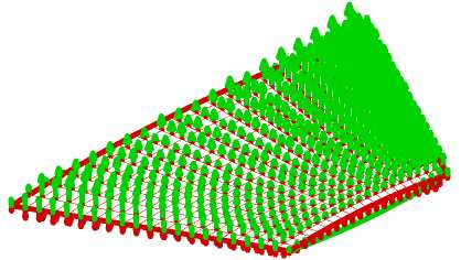
Two methods have been developed to analyze transient loads, the first one is import the mass of Finite Element Method(FEM) node to the CFD/CSD coupling system, we can calculate the aerodynamic force and the inertia force, then can gained the force and moment of structure, show in the figure 7. Another method is load the unsteady aerodynamic force calculate from the CDF/CSD coupling system to the FEM model, make the transient response analysis, we can gained the stress of each part of structure, show in figure 8.

Figure 4. First four elastic mode shapes mapped into CFD surface grid

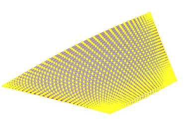
Figure 7. Import the mass of node to coupling system

E

E

aerodynamic inertia

-1000

-2000

-3000

0.00

0.05

0.10

0.15

0.20

0.25

Time(s)

Fi                                                                del

Figure 10. Comparison of bend moment

B. y

Compute the structure response and transient loads at the M∞=2.10,α=2.0, H=2Km, figure 9 shown the general displacement of the fin, structure response is convergence, show that the flight dynamic pressure is lower than the flutter dynamic pressure. figure 10 and figure 11 compared the bend moment and torque of the fin axis cause by aerodynamic and inertia force. Figure12 shows the total bend moment and torque of the fin axis. Figure13 shows the acceleration of the fin. The result show that inertia force plays a significant role in the transient loads, the moment cause by inertia force is lager than the aerodynamic force; because of the huge transient loads, structure may been broken by aeroelasticity under the flutter dynamic pressure.

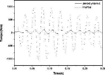
Figure 11. Comparison of torque

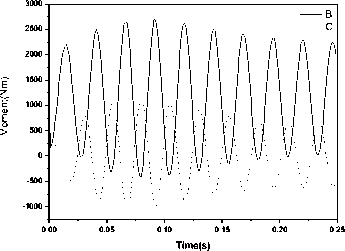
Figure 12. Total of the fin moment

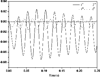
Figure 9. The structure response of the fin

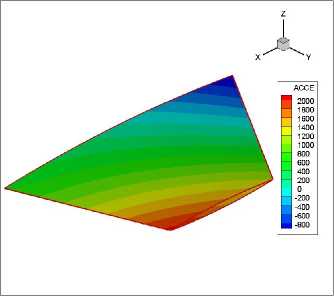
Figure 13. The acceleration of the fin

• V.  F LUTTER WITH PERTURBATION

Aircraft received a variety of perturbation in flight, such as the vibration of engine, the roll of body or the change of attack, these kinds of perturbation will affect the aeroelastic stability of structure. Another low-aspect-ratio fin of missile is selected as a test case. In this work, aeroelastic stability analysis based on CFD/CSD is first identified, and then add vibration movement to CFD/CSD coupling system to identify the influence of perturbation to aeroelastic stability. The structure has two parts of movement, the rigidity movement caused by roll of missile body and the response of aeroelasticity, and the rigidity movement affect the elastic response by the append aerodynamic.

• A.    Flutter with Rolling Perturbation

The roll of the missile body is selected to analyze in this section. The rolling vibration has two parameters, the magnitude of acceleration on the root of fin and the vibration frequency. The vibration adds to the coupling system as a certain structure displacement, the displacement of each node of the fin can be expressed as:

disP = (П/У * DRR * sin( nt) )            (7)

Where:

A is the magnitude of acceleration on the root of fin;

D is the distance of span direction to root of fin;

R is the radius of the missile body;

f is the vibration frequency.

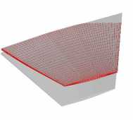
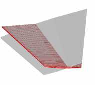
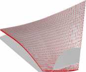
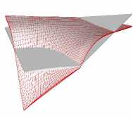
The CFD grid is block structured and uses an C-O topology. This allows points to be focused on the tip region which is most critical for the aerodynamic contribution to the aeroelastic response. View of the CFD grids shown in figure 14. Four mode shapes were retained for the aeroelastic simulation. Table II and figure 15 show the calculated first four fundamental modes and the mode shapes.

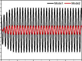
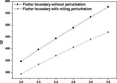
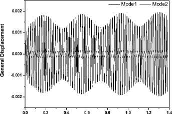
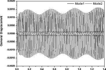
Analyze the aeroelastic response of the fin with perturbation or not based on CFD/CSD coupling separately. The frequency of the vibration is f=66Hz, and the magnitude of the acceleration is A= 1.5G.Qf0 is defined as flutter dynamic pressure without perturbation; Qf1 is defined as flutter dynamic pressure with perturbation. Figure 16_A shows the structure response at the flutter dynamic pressure Qf0 = 347Kpa at 2.0 Mach without perturbation. Figure 16_B shows the structure response at the flutter dynamic pressure Qf1 = 293.5Kpa with perturbation. We can find that the response with perturbation has two frequencies, the flutter frequency (61Hz) and the vibration frequency (66hz), and the response has obvious metronomic, the flutter dynamic pressure is reduced 15.4%. Figure 17 shows the comparison of flutter boundary of fin with perturbation or not, table IV shows the reduction of perturbation to flutter boundary, in the table we can see that the reduction of flutter dynamic pressure by perturbation form 15.4% to 18.6% when Mach from 2.0 to 3.0.

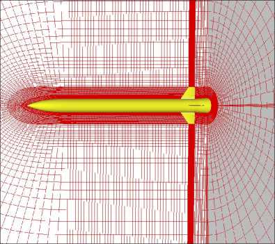
Figure 14_A Slice from volume CFD grid

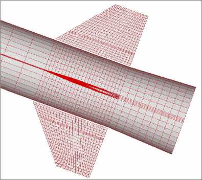
Figure 14_B Detail of surface CFD grid

Figure 14. Viewas of CFD grids

TABLE II.     F REQUENCIES OF THE FIN

Mode	Mode1	Mode2	Mode3	Mode4
Frequency(Hz)	50	75	208	275
Type	Axisbend	Axistorsion	Fin-bend	Fin-torsion

Mode1

Mode2

Mode3

Mode4

Figure 15. Aeroelastic modes for the fin

0.0020

0.0015

0.0010

0.0005

0.0000

-0.0005

-0.0010

-0.0015

-0.0020

0.0              0.1              0.2              0.3              0.4              0.5

Time(s)

图 16_A Response without perturbation(Qf0 = 347Kpa)

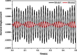
Figure 16_B Response with rolling vibration (Qf1=293.5Kpa)

Figure 16. The comparison of response of the fin at 2.0 Mach

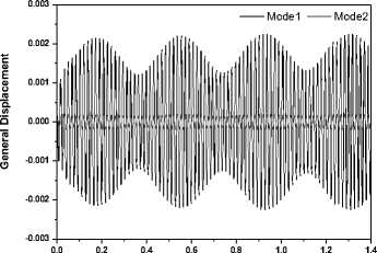
Figure 18 show the structure response of the fin in the 55Hz vibration in different magnitude, we can see that magnitude of the vibration affect the response, magnitude more big the metronomic of the response more evidence.

TABLE IV.    Q F UNDER DIFFERENT PERTURBATION (Q F 0 = 347K PA )

A Qf1(Kpa)X ferq	0.5G	1.0G	1.5G
66Hz	293.5	293.5	293.5
60Hz	287	397	397
55Hz	293	293	293

Time(s)

Mach

Figure 17. The comparison of flutter boundary

TABLE III.    T HE COMPARISON OF FLUTTER BOUNDARY OF THE FIN

Mach	2.0	2.2	2.4	2.6	2.8	3.0
Reduction	15.4%	15.9%	16.4%	17.1%	17.8%	18.6%

• B.    Rolling Perturbation Parameter Influence

In order to analyze the rolling perturbation parameter influence to reduce the flutter boundary, we analyzed three different frequencies and three different magnitude of rolling vibration. The flutter dynamic pressure Qf0 = 247Kpa without perturbation at Mach 2.0, table IV shows the flutter dynamic pressure under different perturbation at mach 2.0, in the table , we can find that the frequency influence the flutter dynamic pressure, the vibration frequency more close to the flutter frequency, the reduction of flutter dynamic pressure more evidence.

Figure 18_A: Response under 55Hz_1.5G vibration (Qf1=293Kpa)

Time(s)

Figure 18_B: Response under 55Hz_1.0G vibration (Qf1=293Kpa)

Time(s)

Figure 18_C: Response under 55Hz_0.5G vibration (Qf1=293Kpa)

Figure 18. Response of the fin in different magnitude

• VI.    C ONCLUSION

Reduced order mode based on Volterra Series is presented to calculate the flutter boundary, and CFD/CSD coupling is used to compute the transient loads. The following conclusions can be drawn from the study: (1) Reduced order mode based on Volterra Series can compute the flutter boundary rapidly and accurately; (2) inertia force plays a significant role in the transient loads, the moment cause by inertia force is lager than the aerodynamic force; (3)because of the huge transient loads, structure may been broken by aeroelasticity under the flutter dynamic pressure.

Perturbation of aircraft will reduce the flutter boundary, The 66Hz_1.5G rolling vibration reduced the flutter dynamic pressure form 15.4% to 18.6% when Mach from 2.0 to 3.0.The frequency influenced the flutter dynamic pressure, the vibration frequency more close to the flutter frequency, the reduction of flutter dynamic pressure more evidence. The magnitude of the vibration affects the response, magnitude more big the metronomic of the response more evidence.

Form the conclusion above can find that, the previous aeroelasticity analysis focus on the flutter boundary in the idea condition is far from enough. Because of the huge transient loads, structure may been broken by aeroelasticity under the flutter dynamic pressure and the perturbation may reduce the flutter boundary, so it is necessary to analyze the aeroelasticity under the compositive force environment.