Chaotic Dynamics of Complex Logistic Map in I-Superior Orbit

Published Online August 2020 in MECS

A mathematician named Verhulst did a major contribution towards the population dynamics by introducing a nonlinear dynamical logistic growth function [1-2]. A demographic evolution encountered after he investigated the Malthus continuous population growth equation. Later, Edward Lorenz [3] identified its significance in chaos theory and used the modified version of Verhulst’s logistic function for his weather forecast model.

The logistic map x_n+1 = rx „ (1 — x „ ) computes the population x lies between 0 and 1 at time n for growth parameter r which was obtained by removing the first term of the logistic equation i.e. x_n+1 = x „ + rx „ (1 — x „ ) [4-5]. The function has wide importance due to the peculiar behavior of r. The same parameter on succession exhibits fixed point, periodic orbit and chaotic behaviour. More precisely, this parameter is responsible for the applicability of the logistic map in various domains like in finance, biological, physics, cryptography, discrete dynamics, fractals, pure and applied mathematics etc [6-11]. The performance of a logistic map in terms of stability or non-stability varies in the orbit at which the iteration method is used to evaluate it. Researchers have been exploring the graphical potential of this map in Picard, Mann, Ishikawa, Noor, and SP orbit. For a detailed study, please refer to [12-15]. According to study, a logistic map has a convergence range 0 < r < 2.75, 0 < r < 4.8999, and 0 < r < 5.4170 in Picard orbit, Mann orbit and Ishikawa orbit respectively. The results demonstrate that the desirable behavior of the logistic map could improvised by iterating it using various iteration methods. Later, extensive research has been conducted by the researcher to explore the logistic map and its various generalization properties [16].

In 2011, the author introduced the modified and extended form of the logistic map and analysed its behavior for the different parameter values [17]. In 2015, the author recognized the importance of a multi-scale population i.e. Mod-LM and proportion of chosen population model i.e. Ex-LM in the superior orbit and observed the extended solution domain for both the functions [18]. But the prior results of LM in Ishikawa orbit encouraged to study the Mod-LM and Ex-LM to get improved results on the stability of the above-said functions. An increased growth control parameter range i.e. r depicts the extended stable trajectories, that coexist with the desirable population dynamics. Although both functions have additional parameters like m,p/y,x , and a where each variable imposed significant impact on the periodic/chaotic dynamics of the corresponding map.

The paper highlights the behavior of Mod-LM and Ex-LM in the I-superior orbit considering control parameter value, convergence point, and chaotic range by varying changeable parameters. In section 2, the background study of proposed work is discussed. The bifurcation diagrams of Ishikawa iterated Mod-LM, and Ex-LM is shown in section 3. In the next section, the experimental approach and results of iterating the functions in an I-superior orbit is discussed. Section 5 exhibits the trajectory map of I-sup LM, I-sup Mod-LM, and I-sup Ex-LM. Also, compared the current approach with the Picard and Mann iterated Mod-LM and Ex-LM functions in section 6. The paper concluded with a summary of findings.

2.    Literature Review

In recent years, many researchers have been analysing the periodic and aperiodic behavior of the logistic map. Later, it’s been realized that by iterating LM using Mann, Ishikawa, Noor, and SP-orbit, chaotic trajectories can be more stabilized for extended control parameter value. Also, the author applied parameter switching theory [19-21] by combining two classes i.e. “extinction + chaos = periodic” and “chaos + chaos = periodic” to get the stable oscillations that coexist with extinction. This switching strategy was revisited in this dynamical system to look for the condition of “chaos + chaos = periodic” in the context of Parrondo’s paradox [22-23]. In 2010 [24], the author applied the Parrondo’s paradox strategy to yield the desirable oscillating outcome of an alternated logistic map from two undesirable chaotic dynamics. In 2011, the author advances the study of chaotic dynamics of an alternated four-seasoned logistic map [25] and also unveil the robustness of the same system using twelve parameters, each reflecting periodic constraints of a month [26]. According to it, an extended Parrondo’s paradox effect using three chaotic parameters yielded “chaos + chaos + chaos = order”.

A pattern of the dynamic behavior of a total of five two-dimensional ecological maps has been examined to find out the periodic oscillation by alternating two parameters associated with chaotic trajectories [27]. Similarly, in ref. [28], a desirable periodic property has been analysed in Beverton-Holt, Ricker, and modified Ricker maps by applying the same switching theory. In ref. [29], not only the switching theory was proved, the author even finds out two new dynamic system situations i.e. “quasiperiodic + quasiperiodic = periodic” and “chaos + chaos = periodic coexistence”. Further, in ref. [30], a desirable ordered outcome is achieved by alternating winter and summer season map functions while the population was driving towards the chaotic and extinction condition individually.

3.    Performance of Logistic Map Variants in Ishikawa Orbit

The present study focuses on the chaotic and non-chaotic behavior of the modified and extended logistic map in I-Superior orbit by analysing their corresponding bifurcation diagram.

• 3.1.    I-Superior Iterates (Ishikawa Superior Iterate)

• 3.2.    I-Superior Modified Logistic Map function

Let’s define function f :X ^X , with X as a set of real or complex numbers. For an initial point x_Q £ X , the Ishikawa or I-sequence of iterates {x „ } will be computed using the given function [31]:

X n + 1 = в ( Уп ) + (1 - в ) x n

Уп = Yf(xn ) + (1 - Y) xn where p and у are positive numbers with condition 0 < p < 1, 0 < у < 1, and 0 < x < 1.

Further, the below section describes the experimental results of I-superior Mod-LM and I-superior Ex-LM in Ishikawa orbit. The experiment is implemented in MATLAB^TM to calculate the minimum and maximum value of growth parameter r for which the considered logistic function remains stable and convergent for all x .

Let’s start by introducing the modified logistic map discussed in ref. [17]. A modified LM was meant to show that the rate of reproduction would be proportional to the power of population depending upon how many partners are contributing towards population growth. The modified logistic map (Mod-LM) was defined as [17]:

^x n + 1 = ^rx m ^{(1 - x} n )

where m > 1 represents the number of partners involved in the growth of population x £ [0,1] in n iterations. The growth rate r is a non-negative real number lies in the interval [r_min, r_max] .

In the present experimental study, an Ishikawa iterated mod-LM function is considered:

X n + 1 = в ( ry m (1 - У„ )) + (1 - в ) X n

Уп = Y( rxm(1 - xn )) + (1 - Y) xn where m,p,y,x are real numbers with m > 1, 0 < P < 1, 0 < у < 1, 0 < x < 1 and re[rmin,rmax]. The function shows the population growth in Ishikawa orbit while m represents the number of partners involved in the reproduction. The function is abbreviated as I-SMLM.

The function I-SMLM analysed to measure the impact on the convergence range by varying the variables value such as m,P,y, and x . In figure 1, three bifurcation diagrams have shown for m = 2,3,4 respectively by considering p, y, and x values constant for all. It can be seen that with increasing m values, the convergence point is extended, but the chaotic dynamics of the map are reduced. Another bifurcation diagram shows the mapping behavior for m = 2,3, ... ,7 in figure 2 to depict the population growth model in case more partners are needed for reproduction. It reveals that the population will collapse early with the increasing m value.

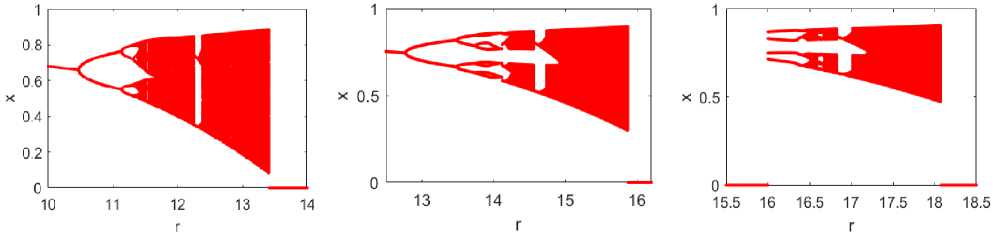
Fig.1. Bifurcation diagram of eq. (4), P = y = 0.3, x = 0.5; (a) m = 2, (6) m = 3, and (c) m = 4, (m = 5 onwards, no bifurcation diagram exist)

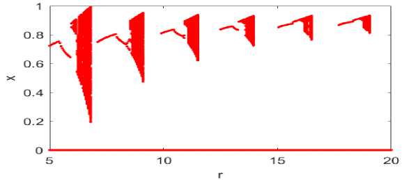
Fig.2. Bifurcation diagram for eq. (4) for P = y = 0.9, x = 0.9, and m = 2,3, ..., 7

• 3.3.    I-Superior Extended Logistic Map function

Another version of the logistic map with two controlling parameters of population growth was proposed to analyse the impact of the function on the reproduction rate known as extended logistic map (Ex-LM). The function is defined as [17]:

x n + 1 =

rxnm a + xm-1

(1 - X n )

here a represents the percentage chosen from the maximum population and varies from 0 to 1. The above function behaves differently for the small population count x < a and nearly saturated population density x ~ 1. The previous case considers very low population density chosen for population growth so it will be heavily dependent on xm. In another case, the reproduction rate will be proportional to x i.e. the population density. An extended logistic map is iterated using the Ishikawa iteration method to obtain more generalized results of population growth model using additional control parameters. The function is defined as:

x n + 1

_{= R} ( ry nm (1 - У п )) ( a + y nm ^-1)

+ (1 - в ) X n

У п = Y

( rx m (1 - X n )) ( a + X nm ^{- 1})

^{+ (1 - Y} ) x n

where m,P,y, x, a are real numbers with m > 1 and re[r_min, r_max]. All other variables are less than unity and have their usual meaning. The function is abbreviated as I-SELM.

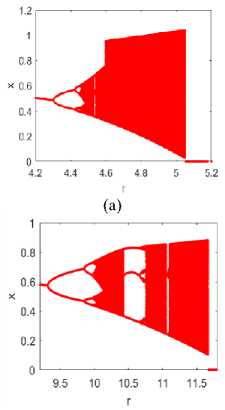
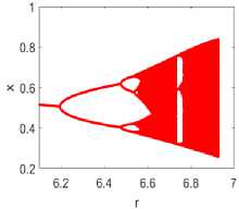
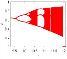
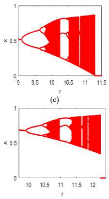
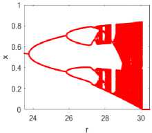
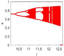
The analysis begins by executing an equation (5) by changing the value of the various variables used. As a result, many bifurcation diagrams have shown in figure 3 to study the impact of each variable on the chaotic dynamics of the map. The first row in the figure shows the map dynamics for P = y = 0.9,0.5,0.3, and 0.1 respectively by considering m, a, and х values constant for all. Similarly, the next row in the figure assumed the value of p, y, a and x constant and shows the map dynamics for m = 3,4,5, 6 respectively. The given figure concludes that the aperiodic behavior is approximately the same as in the previous section for changed p = y values. But does not much impacted by varying m values, which is not aligned with I-SMLM.

(e)

(b)

(f)

(g)

(d)

(h)

Fig.3. Bifurcation diagram of eq. (5), m = 2, a = 0.1, x = 0.5; (a) P = y = 0.9, (6)P = y = 0.5, (с) P = y = 0.3, and (d) P = y = 0.1; and for P = y = 0.3, a = 0.1, x = 0.5; (e) m = 3, (p) m = 4, (y) m = 5, (h) m = 6, (m = 7 onwards, no bifurcation diagram exists)

4.    Discussion

The previous section described the definitions of I-SMLM and I-SELM and also showed their corresponding bifurcation diagrams. Both maps exhibit different characteristics regarding fixed point, periodic and chaotic trajectories and convergence range based on associated changeable parameters. A detailed study of each map is as given below:

Analysis of I-SMLM bifurcation diagram

• 1.    The variation in the control parameter r shows that r_max(m) is approximately equal to r_min(m + 1) for any value of r. See figure 1.

• 2.    Figure 2 shows the bifurcation diagram for m values from 2 to 7. It depicts that the population shrinks if more partners are needed for reproduction which is relevant too.

• 3.    It has been noticed that for x ~ 1(0.6 < x < 1), the population chart exists for m = 2,3,4, ... but for other x values, the reproduction graph can be seen only for m = 2,3, and 4. See Figures 1 and 2. Hence, the population growth model will gradually collapse with less population density and more mating partners.

• 4.    It is evident from table 1 that as m increases, the chaotic range of the map reduces which is shown using the interval range of re[r_min, r_max]. Therefore, the map is more stable in case of the large m values.

• 5.    On the contrary, the chaotic range increases as в and у decrease for the same m value. See Table 2.

• 6.    Also, it has been observed from all table data (refer to table 1 and 2) that the convergence point is extended in case of both decreasing в and у or increasing m values.

• 7.    In the rest of the cases, either map is convergent to a fixed point (single value) or does not exist (NaN).

Table 1. Chaotic range of I-SMLM for x = 0.9, в = Y = 0.9, and changed m values

m	• mtn	r_____ • max
2	5.95	6.85
3	8.4	9.15
4	10.9	11.55
5	13.4	14
6	16	16.55
7	18.6	19.1

Table 2. Chaotic range of I-SMLM for m = 2, X = 0.5 and changed /? and у values

P = Y	^ min	^ max
0.9	6.06	6.82
0.5	8.11	9.05
0.3	11.37	13.42
0.1	29.66	33.48

Analysis of I-SELM bifurcation diagram

• 1.    The bifurcation diagram of various m values has different existential phenomena for different x values. It has been noticed that for x ~ 1, the population chart exists for m = 2,3,4, ... but for other x values, the reproduction graph can be seen only for m = 2,3,4,5 and 6. I-SELM follows the same pattern as in I-SMLM with a minor difference. See figure 3.

• 2.    It is evident from table 3 below that the chaotic range in the bifurcation diagram is almost same for all possible m values i.e. interval range of re[r_min, r_max]. Whereas in I-SMLM, the interval range of dynamic sessions does not overlap with increasing m values.

• 3.    In the case of changing в and y, the outcome of a chaotic range in the bifurcation diagram of I-SELM is the same as in I-SMLM. The system dynamic has extended as в and у decrease for the same m value. See Table 4.

• 4.    The convergence point does not change much in case of increasing m values while extending in case of decreasing в and Y- But it will intact with varying initial value x. (See table 3 and table 4).

• 5.    The changed m value does not affect the chaotic range (r_max — r_min), whereas considering an increased percentage of the population (a) shift the convergence point slightly farther. Therefore, the dynamic behavior of the map extends with a large number of populations cut-off. Refer to table 3 and table 5.

• 6.    In the rest of the cases, either map is convergent to a fixed point (single value) or does not exist (NaN).

5.    Chaotic Performance in terms of Trajectory

Table 3. Chaotic range of I-SELM for x = 0.5, a = 0.1, в = y = 0.3, and changed m value

m	T - . * mtn	T _ _ * max
2	9.096	11.29
3	9.320	11.67
4	9.592	11.95
5	9.928	12.24
6	10.33	12.58

Table 4. Chaotic range of I-SELM for m = 2,a = 0.1, X = 0.5 and changed /? and у values

P = Y	^ min	? max
0.9	4.45	5.05
0.5	6.55	6.92
0.3	9.80	11.29
0.1	27.52	30.07

Table 5. Chaotic range of I-SELM for m = 2,X = 0.5, /? = у = 0.3, and changed a values

a	* mtn	* max
0.04	8.46	10.40
0.1	9.09	11.28
0.3	11.23	14.14
0.5	13.35	16.92

A trajectory of a chaotic map represents the path followed by the function upon iteration. The sensitiveness of the function on its initial condition is analysed by tracing the phase space of the approximately closed points. As much the function shows diversity towards it, mapping depicts more randomness in its chaotic behavior. The below figure 4 shows that as compared to I-superior logistic map, I-superior modified logistic map and I-superior extended logistic map cover more phase space. Hence the complex form of the logistic map renders more ergodicity and better randomness property.

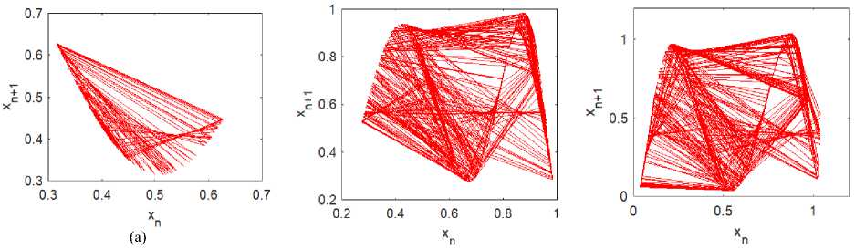
(b)

(c)

Fig.4. Trajectory diagram (a) I-Superior Logistic Map, (b) I-Superior Modified Logistic Map, (c) I-Superior Extended Logistic Map

6.    Comparison between Picard, Mann and Ishikawa iterated Modified and Extended logistic map

In Table 6, the convergence of logistic map variants to a fixed point has been computed in all three iteration methods (i.e. Picard, Mann, and Ishikawa). However, the number of changeable parameters is different for each map and also for each iteration method, so the comparison between iteration methods is shown by assuming the same variable as constant. For example, in the case of a modified map, the value of m,x₀,p &  у are constant as required throughout the analysis. Similarly, the value of m, x₀, a, P & у of the extended logistic map are constant in all iteration methods. The result shows a better stable dynamic of both a Mod-LM and the Ex-LM as compared to the logistic map. Subsequently, the iterated modified and extended maps also have an enhanced desired stable outcome. The study concluded with two points:

• 1.    In the case of a modified and extended logistic map, the convergence point stretched in Mann and, then gradually in Ishikawa iterate. (See results row-wise).

• 2.    Whereas, extended logistic map converges fast as compared to a modified logistic map for each iteration method. (See results column-wise).

7.    Conclusion

Table 6. Comparison between modified and extended logistic map in various orbits

Type of Logistic Map	Picard	Mann	Ishikawa
Modified Logistic map (X o = 0.5)	0 < r < 5.328 (m = 2)	0 < r < 5.78 (m= 2,p = 0.8) 0 < r < 9.75 (m= 2,p = 0.3)	0 < r < 6.06 (m = 2,p = у = 0.8) 0 < r < 10.47 (m = 2,p = у = 0.3)
Extended Logistic map (x0 = 0.5)	0 < r < 3.2329 (m = 2, a = 0.04)	0 < r < 3.75 (m = 2,p = 0.8, a = 0.04) 0 < r < 8.05 (m = 2,p = 0.3, a = 0.04)	0 < r < 4.196 (m = 2,p = у = 0.8, a = 0.04) 0 < r < 8.456 (m = 2,p = у = 0.3, a = 0.04)

The paper examined the chaotic behavior of Mod-LM and Ex-LM in the I-superior orbit using three and four controlling parameters respectively. The main elements to analyse each iterated map include critical points and chaotic range on the bifurcation diagram by varying the parameter values of the complex logistic map functions.

The experimental study states that the convergence point extended to decreasing p & у values and for increasing m value in I-SMLM. It’s also evident that for increasing m values, the interval range of r quickly convergences. Hence, it reduced the chaotic influence of the said logistic map. On the other hand, the I-SELM does not much change its convergence point for increasing m. The chaotic range of I-SELM improves either by decreasing p & у values or with a large number of populations cut-off i.e. a. The analytical report signifies that in the case of a large number of mating partners (m), a higher population (x) is needed to support the population growth parameter. As with increasing m, the range of growth parameter r is also increasing. It has also observed that if a population growth model has a smaller number of the population and required large mating partners for reproduction, the ecological system can collapse because of the parameter region shrinks. Moreover, the iterated output described the stability domain of each map which lead the given map to the study of nonlinear phenomena. In the future, the chaotic nature of I-SMLM and I-SELM can be further explored to generate fascinating fractal images to be used in real-time applications.