Characteristic Research of Single-Phase Grounding Fault in Small Current Grounding System based-on NHHT

Published Online December 2016 in MECS

At present, the most widely used signal processing method is Fourier transform, but since Fourier transform can only be applied to linear superposition of FM signal, it can not do time frequency analysis, in order to solve this problem, wavelet transform came into being.

The wavelet transform proposed by Morlet et al., through the expansion and translation of the signal to carry out multi-scale decomposition, can effectively obtain all kinds of time-frequency information from the signal, it has good localization property in time domain and frequency domain, and has the characteristic of multi-resolution analysis.

However, wavelet analysis is not adaptive, once the wavelet base and the decomposition scale are chosen, it is used to analyze the data with multiple frequency components, the results can only reflect the signal characteristics of a fixed time-frequency resolution, and wavelet analysis is not suitable for non-stationary data.

A new signal processing method -- Hilbert Huang transform[1], is proposed for the non-stationary signal by Norden E. Huang et al. In 1998, this method is considered to be a major breakthrough in the linear and steady-state analysis of the Fourier transform.

Norden E. Huang at first proposed the HHT to analyze ocean current signal and wave signal data, and proved its advantages in the analysis of non-stationary and nonlinear signal processing field. Since then, he has used HHT to analyze seismic wave data, which greatly inspired many earthquake researchers and applied it to the field of earthquake research[2-3].

The application of HHT is very extensive, such as Analysis of earth's inner force wave in the field of geophysics[4], structural identification and modal analysis in structural analysis[5], the analysis of solar radiation changes in the field of astrophysics[6], the estimation of Teager energy by using the Hilbert–Huang transform[7], and in [8], HHT is used as an adaptive method to study their multiple scale dynamics in Marine environmental time series, and so on. Its good timefrequency characteristics are demonstrated.

In the field of fault processing, the applicability of Hilbert–Huang transform (HHT) for internal leakage fault detection in valve-controlled hydraulic actuators is investigated in [13], the HHT is proposed to detect the very early stage fault in interturn insulation by only analyzing the stator current in the PMSWG in [14], fault detection is realized by means of HHT of the stator current in a PMSM with demagnetization in [15]. Also, Wavelet and Artificial Neural Networks are used to Fault diagnosis [16-17].

In the field of energy, Hilbert spectral analysis (HSA)

is used to characterize the time evolution of non-stationary power system oscillations following large perturbations in [18], also HHT is used to analyze the nonstationary power-quality waveforms in [19].

The core part of HHT algorithm is empirical mode decomposition (EMD). In essence, EMD is to gradually decompose the oscillation mode or trend of different scale in signal, and produces a series of time series with different characteristic scales, and each time is an IMF component of intrinsic mode function. With the help of Hilbert transform (HT), the time spectrum of signal can be further obtained, which can accurately reflect the timefrequency characteristics of the signal.

In the system of 3 ~ 66kV power system in which the neutral point is not connected to ground or connected to ground through the arc suppression coil, when the ground fault occurs in a certain phase, because the short circuit can not be formed, the fault current is often much smaller than the load current, this phenomenon is called "small current grounding system". The practice shows that the occurrence of single-phase grounding fault in the power grid is the highest, which is about 85% of the total failure of the system.

Because the fault current is small in the small current grounding power system, and the detection is difficult, and has not been well solved, which has become one of the research hotspots in this field. In this paper, HHT is used to analyze the fault current of single-phase ground fault in small current grounding system.

The main research work of this paper is as follows:

• (1)    The transient analysis of the grounding current is carried out and the influence factors are analyzed, the grounding current is mainly transient capacitance current and transient inductance current, but because of the difference between the two frequencies, it can not be offset each other.

• (2)    The empirical mode decomposition (EMD) process and the normalized Hilbert transform (NHT) algorithm are presented. The NHHT is used to analyze and verify the nonlinear and non-stationary amplitude modulation signals.

• (3)    Under the EMTP_ATP environment, a small current grounding system is built, and the parameters of the system are calculated, and the single-phase grounding fault is simulated.

• (4)    Extracts transient signal, use HHT to analyze transient current signal, and obtain time spectrum and Hilbert marginal spectrum of Zero sequence transient current signal of fault feeder, and the influence of the fault phase and the grounding resistance on the timefrequency characteristics of the signal is analyzed.

• II.    T RANSIENT ANALYSIS OF S INGLE P HASE G ROUNDING

F AULT IN S MALL C URRENT G ROUNDING SYSTEM

When single phase grounding fault occurs in the neutral point via the arc suppression coil grounding grid, transient capacitance current and transient inductance current constitute the transient grounding current flowing through the fault point. But because of the difference between the two frequencies, the transient process can not compensate for each other. The equivalent circuit of system transient current for the neutral point via the arc suppression coil grounding grid is shown in Fig.1.

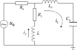
Fig.1. Transient equivalent circuit of single phase grounding fault

In Fig.1, C is the equivalent capacitance of the grid to the ground, L is the equivalent inductance of the circuit, power supply, and the transformer in the zero sequence circuit. R is the equivalent resistance of the zero sequence circuit, including the grounding resistance of the fault point and the arc path resistance. R and L are respectively the active loss resistance and inductance of the arc suppression coil, u is zero sequence power supply voltage.

• A. Transient capacitance current

Since the self vibration frequency of the capacitance current is generally higher, and the inductance of the arc suppression coil is L » L_n, so the influence of R_L and L in Fig.1 is neglected in analyzing its transient characteristics. By using the equivalent circuit of L_o &  C_o &  R _o and the system zero sequence voltage source u₀ = и_фm sin( ro t + ф ) , transient capacitance current i_c can be obtained. From Figure 1, the differential equation can be got:

d i      1 t

R_ni_r + L_n —C +-- i_r d r = u_ft

^{0 C 0} d t   C _o ^J 0 C       ⁰

When the grounding resistance is very small, at R < 2^Lo/Co , the system is in a state of under damping condition, the transient capacitance current has a periodic oscillation and attenuation characteristics. Transient self vibration component i    and steady state power frequency component i      constitute transient capacitance current i , by using the relationship between iC.os + iC.st = 0 and ICm = U$m^C0 at initial conditions t = 0, the following equation can be got by Laplasse transformation:

i C =

= I.

Cm

^{f ro}f •                                          -fit

I -^sin ^ sin ro t - cos ^ cos ^ t I e к ro                             ^f )

+ cos( ro t + ф )

In the formula (2): U is the amplitude of the phase voltage, i _Cm is the amplitude of the capacitor current, to y is the transient self-vibration angular frequency, § = 1 т = R/ L _o/2 is the attenuation coefficient of free oscillating component, where the т is the time constant of the loop. When т is larger, the self - vibration attenuation is slower, whereas, the attenuation is faster.

By analyzing formula (2), if the single phase grounding fault occurs in ф = П 2, and at t = T_f /4 ( T_f = 2 n/to_f is self vibration period), the amplitude of the self vibration part of the capacitive current is the maximum i :

Vl = ^ st ^ L ^|co^s< ф + § ) e

- cos( to t + ф + § )]

In the formula (6): ^ = ифт(toW) is the steady state flux, § = arctan[RL (toW)]  is the phase angle of compensating current, Z = Д R2 + (toL)2  is the arc suppression coil impedance, т is the time constant of the inductance loop. Due to rl toLoL , take Z « toL , § = 0. In consideration of у =Vos +^st, к = 4. + + 4« os        st                c        st and I  = ифтJto>L)) , the expression of the transient inductance current i can be obtained as follow:

T f

_T   ^to f   4 T_c

= ICm —e C to

If the single phase grounding fault occurs in ф = 0, and at         , the minimum value of        for the self f                                             C.os min vibration current is:

L.

C.os min

I Cm

to

e

—

T f

2 T _C

to

Self-vibration frequency to of self-vibration current is:

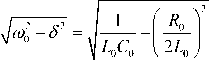
In formula (2), Self-vibration frequency of the loop is to = VV LJC • When the grounding resistance increases to R >  2 ^ LjC , the system is in a state of over damping state, and the loop current has a non periodic oscillation attenuation characteristic and tends to be stable.

According to the above analysis, the change of the fault resistance has a great influence on the transient characteristics of the grounding system of the neutral point via arc suppression coil.

B. Transient inductance current

Differential equation of the core flux can be derived from Fig. 1 [1]:

- 1

i_L = I_Lm [cos фе^т - cos( tot + ф )]                ⁽⁸⁾

By the formula (8), it is known that the transient DC component and the steady-state AC component constitute the transient inductance current i , and the initial amplitude of the transient DC decay process is related to the phase ф , the attenuation coefficient is determined by loop impedance. Transient DC component in the ф = 0 is the largest, and in the ф = П 2 is the smallest.

C. Transient grounding current

System transient grounding current is composed of transient capacitance current i and transient inductance current i , although the amplitude difference between i and i is not large, they are in different frequency bands and can not compensate for each other.

The expression of the transient grounding current i can be derived from the formula (2) and (8):

i d = i C ⁺ i L = ⁽ I Cm - I Lm ) ^coS^{( tot +} ф)

( to _f

+ Icm\    sin ф Sin tot - cos ф cos tot

( to                              ^f

tt

-- -- e Tc + Ilm cos фе 4

u ₀ = R_Li_L + W d ^L-

d t

In the formula (6), W is the turns of the arc suppression coil, and у is the core flux of the arc suppression coil.

Before the grounding fault, no current flows through the arc suppression coil, that is, _фг is zero. Take i = w ^_L L into formula (6), _Фь expression can be obtained as follow:

In the formula (9), the first part of equality right is the steady-state component of the grounding current, the amplitude is the difference between the amplitude of the steady state capacitance current and the steady state inductance current, and is closely related to the fault phase ф , frequency is power frequency. The other part is the transient component of the grounding current, which is composed of two parts, transient free oscillation component of capacitance current and DC decaying component of inductance current.

From the above analysis, after the occurrence of a single phase grounding fault, transient grounding current flowing through the fault point contains transient capacitive current component of damped oscillation and the decay transient inductance current component. Whether the system is operated in the neutral point via

the arc suppression coil grounding mode or not grounding mode, the transient capacitance current dominates the amplitude and frequency of the transient grounding current, and its amplitude is also related to the fault phase. The initial value of DC component in the transient inductance current is related to the initial phase and core saturation.

• III.    H ILBERT H UANG TRANSFORM (HHT)

• A.    Instantaneous frequency and intrinsic mode function (IMF)

Instantaneous frequency is one of the most important concepts in time frequency analysis. The definition of instantaneous frequency is needed to satisfy a certain condition, and not all the instantaneous frequency of the signal has a physical meaning, only when the signal is approximated by a single component signal, each moment corresponds to a single frequency component, the instantaneous frequency has the actual physical meaning. In order to obtain the instantaneous frequency of physical meaning, Norden. E. Huang et al. proposed the concept of intrinsic mode function (IMF).

Using Hilbert transform to analyze the intrinsic mode function (IMF) can get good time frequency characteristics, but most of the signal is not the intrinsic mode function (IMF), and is the combination of the many of intrinsic mode function (IMF). Therefore, the correct time frequency characteristics can not be obtained directly through the Hilbert transform, so that we can not accurately analyze the signal directly. In order to use the Hilbert transform to analyze the nonlinear and non-stationary signals correctly, the signal is decomposed to IMF at first, then the empirical mode decomposition (EMD) is developed.

• B.    The principle of empirical mode decomposition (EMD)

Empirical mode decomposition (EMD) uses selection after layer by layer, and get a series of intrinsic mode functions (IMF), and the dominant frequency of the intrinsic mode function (IMF) is lower and lower, the dominant frequency of IMF obtained firstly is the highest, and the IMF obtained lastly is the lowest, therefore, it is essentially a filter bank.

If a signal with random noise is decomposed by the empirical mode decomposition (EMD), the high frequency intrinsic mode function (IMF) component is usually a high frequency noise of the signal, and the residual signal component is usually the mean or trend of the original signal. Each intrinsic mode function (IMF) component obtained from decomposition has obvious physical meaning and contains a certain range of characteristic scales.

The intrinsic mode function (IMF) must meet the signal of the following two conditions [1]:

envelope which are determined by local maximum point and local minimum point is zero, that is, the signal is locally symmetric about the time axis. IMF is essentially a narrow band signal.

Because any given signal can not satisfy the IMF condition, the complex signal is decomposed into a series of IMF by EMD[20]. For a given signal X ( t ), the EMD process is as follows[21]:

Step1. finds out all the local maxima and minima of X ( t ), by using the three spline interpolation, the local extreme value is connected to the upper and lower two envelope of e ( t ) and e ( t ). X ( t ) minus the mean m i ( t ) of the envelope, m 1 ( t ) = ( e J t ) + e^.t ))/2 , ^and the first component h ( t ) = X ( t ) - m_x ( t ) is obtained.

Step2. check whether h ( t ) is IMF. If not, then return to step 1, and take h ( t ) as a new signal for screening. Repeat screening k times, until h ( t ) becomes IMF, take c_v ( t ) = h_v ( tt ) . Residual signal is r ( t ) = X ( t ) - c ( t ) .

Step3. take r ( t ) as a new signal, re perform step 1 to 2, get the new IMF _c ( t ) and the residual volume _r ( t ). Repeat iteration n times: r ( t ) = r ^t )- c_n ( t ), until r ( t ) is a monotonic function, EMD is over.

EMD is an adaptive filtering process, and the signal is decomposed adaptively according to the frequency scale, a series of narrow band signals are obtained from large to small frequency. Due to the completeness of EMD, the original signal X ( t ) can be expressed as the sum of n IMF and an average trend component r ( t ).

• C.    The normalized Hilbert Huang transform (NHHT)

The normalized Hilbert- Huang transform (NHHT) is an improved Hilbert- Huang transform (HHT), it is composed of empirical mode decomposition (EMD) and normalized Hilbert transform (NHT).

For any continuous time signal X ( t ) , Hilbert transform is as follow:

y ( t ) = 17 X T )^        (10)

n J t — T

—^

X ( t ) and Y ( t ) form complex conjugate pairs, and constitute an analytical signal as follows:

Z ( t ) = X ( t ) + jY ( t ) = 7 X ²( t ) + Y ²( t ) e j ^{6 (} t )          (11)

₉ ( t ) = arctan Z ( t l                     (12)

X ( t )

According to the derivative definition of the analytic signal phase, the instantaneous frequency is as follow:

_{f ( t ) =} 1 d θ ( t )                          (13)

2 π  d t

It can be seen that f ( t ) is a single valued function of t , the frequency changes with time, in order to make the instantaneous frequency meaningful, the time series of the Hilbert transform must be monotonous, and the IMF after the EMD just meets the requirement.

The definition of Hilbert spectrum (united timefrequency amplitude spectrum)[22] is:

kk

H(ω,t)=Re∑z(t)=Re∑a (t)ejθi(t)

i=1

Hilbert marginal spectrum[23] is:

H(ω)=∫TH(ω,t)dt(15)

In the formula (15), T is the signal length. Based on the H ( ω ,t) energy distribution in time frequency space, the energy (amplitude) of all moments for a certain frequency is added to form the total energy (amplitude) of the signal, that is, the Hilbert marginal spectrum H ( ω ). But the frequency is not always present at all time, or only at a certain moment, it may appear several times in different or equal amplitude, this physical meaning is consistent with the physical meaning of the Fourier spectrum[24], but in the Fourier spectrum, the same magnitude is required for any frequency, which is easy to destroy the true frequency of the signal and appear false frequency.

Because of the limitation of Bedrosian principle, the amplitude can cause serious disturbance to frequency modulation, which affects the instantaneous frequency. In order to eliminate this limitation, a normalized algorithm is adopted to decompose IMF into a unique empirical envelope (AM) and a carrier (FM), and then Hilbert transform for carrier is done for Instantaneous frequency[25]. The essence is a kind of reverse frequency modulation and amplitude modulation. Specific steps are as follows:

Step1. The maximum value of the absolute value of each IMF component is solved, and the endpoint is also regarded as an extreme value.

Step2. The three spline is used to fit the maximum value curve e ( t ). When the envelope is lower than the original data sequence, the local area envelope is replaced by a straight line envelope, use envelope normalized data f = imf e , f is used as the new IMF.

Step3. Repeat steps 1, 2 until the absolute value of IMF is no more than 1, and eventually will obtain its frequency modulation (carrier) component f and amplitude modulation components a ( t ) = e ∗ e ∗  ∗ e .

Step4. In order to obtain the instantaneous frequency, the Hilbert transform is carried out for the carrier.

United time-frequency amplitude spectrum of the signal is obtained based-on amplitude modulation component and instantaneous frequency, and then the Hilbert marginal spectrum is obtain.

• D.    Analysis of an example

As a time-frequency analysis method, of course, NHHT is most commonly used in nonlinear non-stationary signal analysis. Use NHHT to analyze nonlinear and non-stationary AM and FM signal in the formula (16):

Y = sin(30 π t ) + 10 t cos(70 π t + sin(20 π t )) + sin(30 π t ² ) (16)

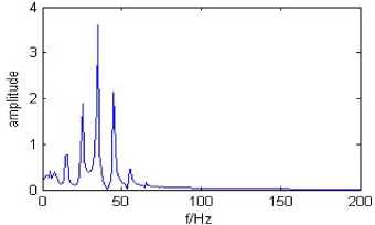
Fig.2. Fourier spectrum of the simulation signal

Use NHHT to analyze the signal, firstly EMD (Fig. 3) is done, the original signal is decomposed into a series of IMF and residual RES, IMF is a series of signal components with different frequency components. According to the approximate orthogonality of EMD, the IMF is nearly orthogonal to each other, that is, the frequency components of each IMF component are almost different.

In Fig.3, each IMF is arranged according to its frequency components from the big to small arrangement, and due to the residual RES is very small, the decomposition is more successful. Seen from Fig.3, the signal is made up of three parts: the 15Hz constant frequency component, linear frequency modulation component, as well as frequency oscillation component by taking 35Hz as the center and 10Hz as the oscillation amplitude.

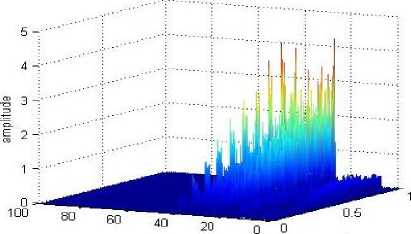
NHT is done for the IMF obtained by EMD, and united time-frequency amplitude spectrum (Fig.4) is obtained. In the united time-frequency amplitude spectrum, the amplitude changes of the same frequency can be seen at different times, this is not done in the Fourier analysis which is required to be based on the same frequency and its amplitude can not be changed with time.

Seen from Hilbert marginal spectrum (Fig.5), there is no more than 50Hz frequency band, and the frequency components of 55Hz appear in the Fourier spectrum. According to the theoretical analysis, in a second the signal frequency can not be greater than 50Hz, the false frequency appears in the Fourier spectrum, actual results show that the FFT is not suitable for analyzing nonlinear signals and appear spectrum leakage, and NHHT is not restricted, these show, compared to FFT and other conventional algorithms, NHHT in analyzing nonlinear signal has incomparable superiority.

Empirical Mode Decomposition

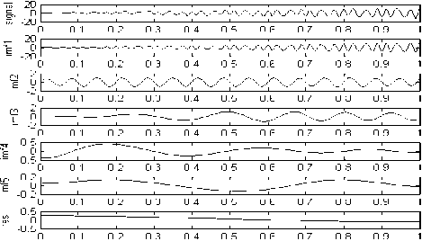
Fig.3. EMD of the simulation signal

№                 1/8

Fig.4. United time-frequency amplitude spectrum of the simulation signal

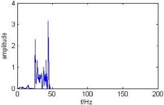
Fig.5. Hilbert marginal spectrum of the simulation signal

• IV.    S IMULATION AND A NALYSIS OF S INGLE P HASE G ROUNDING F AULT

• A.    Construction of single phase grounding fault system

EMTP is the first of the electromagnetic transient analysis software produced by Tan Weier, Canada, which is a powerful tool for power system simulation, which can be used to  analyze  the  steady  and  transient characteristics of power system. The typical application of EMTP is to simulate the change of electrical parameters with time under the disturbance in power system, such as the change of the feeder current after the occurrence of grounding fault in the power grid.

ATP is the program package programmed by the Danish scholar Hart based-on the use of EMTP for the kernel. Because ATP uses the Windows interface, it has a more friendly man-machine window compared with the traditional EMTP, the application is more simple. In ATP, the simulation of 5 output lines is built, and the topological structure of the model is shown in Fig.6.

Fig.6 simulation model is a 10kV three-phase symmetric system model, the line uses the distribution parameters module with 5 outlets. In Fig.6, 10kV voltage is obtained by 110kV AC 3 phase power supply through the 110/10kV transformer, the transformer is Yy0. It is not the grounding system when the K is open, and is the grounding system through the arc suppression coil when the K is closed.

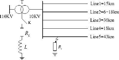
Fig.6. Simulation model of small current grounding fault

In Fig.6, the parameters of the small current fault grounding system are shown as follows: Line L1 is 15km pure cable line. Line L2 is a mixed line of overhead line and cable, the length of which is 18km and 6km respectively. L3, L4 and L5 are the pure overhead lines, the length of which is 30km, 18km and 43km.

Cable line parameters are:

Positive sequence impedance Z_v = (0.125 + j 0.095) П /km , Zero sequence impedance Z _o = (0.97 + / 1.590) 0 /km .

Positive sequence susceptance b_v = 83.566 ^5 /km , Zero sequence susceptance b ₀ = 83.566 ^ 5 / km .

The parameters of the overhead line are:

Positive sequence impedance Z = (0.270 + j 0.351) 0 / km , Zero sequence impedance Z _o = (0.475 + j 1.757) O / km .

Positive sequence susceptance b = 3.267 д $ /km , Zero sequence susceptance b ₀ = 1.100 ^ 5 / km .

The terminal load of each outlet is 1000 + j 20 0 .

The capacitance current of single phase to ground can be calculated as follow:

I c = 3 ® C 0 jJ^ = 32.46(A) >  20(A)            (17)

In general, when the capacitance current is more than 20A in the 10KV medium voltage power grid, it is necessary to install the arc suppression coil. The inductance of the arc suppression coil is obtained by using formula (18):

n % ® L =

3 ® C 0.

The arc suppression coil is set by the over compensation of n % =110%, through calculation, the inductance of arc suppression coil is L =0.55H. The value of series resistance is set to R =17.28 Q by the 10% arc suppression coil inductance.

• B.    Time frequency analysis of zero sequence transient current based on HHT

• 1)    Extraction of transient signal

From the previous analysis, the transient grounding current includes the steady state power frequency component and transient component of grounding current. According to the superposition principle, the power frequency component in the fault transient zero sequence current of each feeder is the superimposition of the asymmetric component before the fault and the steady state power frequency component after the fault. And because the actual small current grounding fault occurs after the 5~6 cycle, as shown in Fig.7 (a), the zero sequence current transient component has been quite small, it is considered that the electromagnetic transient process is basically the end. Therefore, a reasonable time window is designed to filter the steady-state component, its window size is a power frequency cycle, the expression of the zero sequence current transient component is as follow:

i0 kf ( t ) = i 0 k ( t ) - i 0 k ( t + 7 T )                 (19)

In the formula (19), i ( t ) is the zero sequence current of the k feeder, and T is the power frequency cycle.

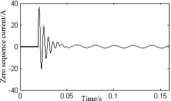
(a) The zero sequence current of fault line

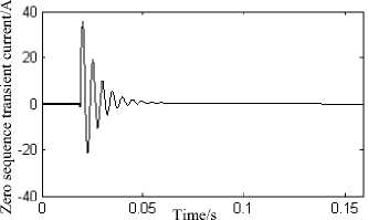
(b) The Zero sequence transient current of fault line

Fig.7. The extraction of fault signal transient component

In Fig.7 (a), the grounding fault occurs in the feeder L5 at the bus terminal 12km and the fault phase 600, the ground resistance is 2 Q . The actual zero sequence current flows through the feeder L5, which contains the steady state and transient components. Can be seen after the above treatment, it is very good to filter out the steady-state component of the fault current, the transient component is obtained as shown in Fig.7 (B).

• 2)    Transient time frequency analysis of zero sequence transient current

HHT is done for the zero sequence transient current signal in Fig.7 (b). First, EMD is done for the zero sequence transient current, seen from Fig.8 (a), the current signal which contains a variety of frequency is decomposed into a series of different center frequency current components, namely IMF1 to IMF6, its time scale is getting bigger and bigger, that is, the center frequency of each IMF frequency band is gradually reduced. The center frequency and bandwidth of each current component are adaptive, without a priori decomposition basis function, the frequency components of each IMF component are not equal in theory, and the amplitude of each IMF component is determined by its time and frequency. From the ratio of the EMD residual amplitude and the original signal, the decomposition is more successful. From Fig.8 (a), the main frequency components of the signal are concentrated in IMF4, the amplitude of the other IMF components are very small which compared to IMF4, also the frequency is about 190Hz by Hilbert transform for IM4, which is relative to the Hilbert marginal spectrum of Fig.8 (c).

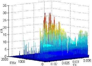
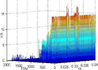
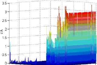
The united time-frequency amplitude spectrum is obtained by the normalized Hilbert transform (NHT) for the IMF component of the decomposition, that is, the Hilbert spectrum (Fig.8 (b)). From Hilbert spectrum, it can be seen that the distribution of the frequency components of the transient current in the whole time frequency space, the main frequency band of the transient current is concentrated in the low frequency band between 0 and 500Hz. The high frequency components of the frequency components are relatively scattered and mainly concentrated in the moment of failure occurrence. In the Hilbert spectrum, the amplitude is smaller but the power frequency steady-state periodic component is found in the whole analysis. This corresponds to IMF6 after EMD. From Fig.8(a), it can be seen the frequency of IMF6 is 50Hz, and the analysis of the transient current in the last part shows that this is the function of the system inductance. The Hilbert spectrum shows that the signal is attenuated in the whole, and the performance of the first 1/4 power frequency cycle is obvious, which is consistent with the transient component of zero sequence current.

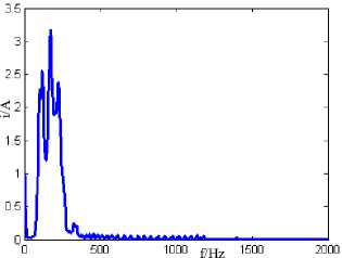
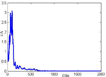
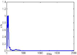
The amplitude spectral of Hilbert is integrated in the whole analysis, and the amplitude of each frequency component at each moment is accumulated, the Hilbert marginal spectrum is obtained. This is a kind of spectrum of signal energy distribution, it is a kind of characterization form of frequency and energy, and the amplitude will be normalized in the practical application. Seen from Fig.8 (c) of the Hilbert marginal spectrum, its frequency components are relatively concentrated around 200Hz, the main energy distribution of the signal is between 0-500Hz.

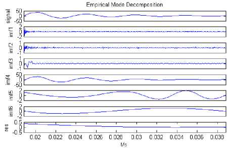
(a) Empirical mode decomposition of zero sequence transient current

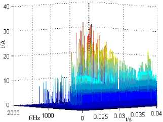
is changed at fault line (L5). From the graph, we can know that with the increase of the fault phase, the DC component of the current decreases rapidly, and the amplitude of the current is obviously increased, which is consistent with the conclusion of the theoretical analysis. It can be seen from the Hilbert spectrum of different fault phase, the amplitude of the main vibration mode of the current signal is exponential decay with the increase of time. With the increase of the phase, the frequency components of the current are becoming more and more abundant, and the marginal spectrum of Hilbert describes this phenomenon in the frequency domain.

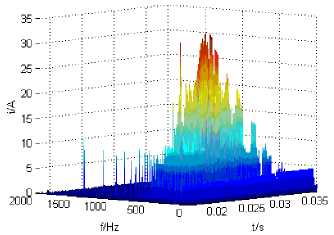
(b) United time-frequency amplitude spectrum of zero sequence transient current

14 -г

4---

0-I—-^^^

2000       1000

f/Hz

0 02   0 025 t/s

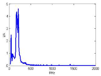
(c) Hilbert marginal spectrum of zero sequence transient current

Fig.8. Transient time frequency analysis of fault line (L5) zero sequence current

• (a) Hilbert amplitude spectrum at 00

• 2.5-----------------------,-----------------------,------------------------,------------------

f/Hz

(b) Hilbert marginal spectrum at 00

25-г

20-■

C. The influence of main factors on the transient timefrequency characteristics

The main factors that affect the fault signal are the structure of the circuit, the fault phase, the grounding resistance, the distance between the fault point and the bus, among them, the fault phase and grounding resistance are the dominant factors. In this paper, the effects of the fault phase and the grounding resistance on the time-frequency characteristics of the signal are discussed.

1) The influence of the fault phase on the transient timefrequency characteristics

Under the condition of grounding resistance 5, by changing the fault phase, the zero sequence current of a series of fault feeder (L5) is obtained. The transient component is obtained by the previously designed filter window, the time-frequency characteristics of the current signal are obtained by HHT analysis, as shown in Fig.9.

Fig. 9 is time frequency characteristics of the transient component of zero sequence current when the fault phase

15 <

2°0° 1500 woo f/Hz

0.02 0 025t/s

(c) Hilbert amplitude spectrum at 300

2----------------------------------.----------------------------------.----------------------------------.-------------------------------

f/Hz

(d) Hilbert marginal spectrum at 300

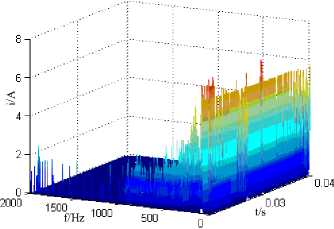
(e) Hilbert amplitude spectrum at 600

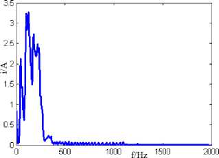
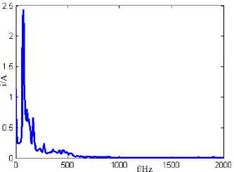
(f) Hilbert marginal spectrum at 600

(g) Hilbert amplitude spectrum at 900

(h) Hilbert marginal spectrum at 900

Fig.9. The influence of the fault phase on the transient time-frequency characteristics of fault line zero sequence current

In short, with the increase of the phase, the amplitude and frequency components of the signal increase, the distribution of the signal energy will be more and more dispersed.

• 2)    The influence of the grounding resistance on the transient time-frequency characteristics

In [26], the effects of very-high resistance grounding on the selectivity of ground-fault relaying are studied.

The fault resistance and fault phase are the main factors that affect the zero sequence current. Set the fault phase at 90 ⁰ , change the grounding resistance, analyze the signal time-frequency characteristics of different grounding resistance.

Fig.10 is Hilbert spectrum and Hilbert marginal spectrum of the fault line at 50Ω , 100Ω , 500Ω , 5000Ω . It can be seen from the figure that with the increase of grounding resistance, signal current amplitude and frequency components gradually reduced. At the 50 Ω around, the system has been in a state of damping, and the frequency components of the system are relatively concentrated in Fig.10 (b). And with the increase of the grounding resistance, the system is re entered into an under damping condition, as shown in Fig.10 (d), although the main frequency components of the system are concentrated in 50Hz, but the energy of 150Hz and 250Hz is also larger, and the system energy is relatively dispersed. After a further increase in the grounding resistance, the current signal frequency is further concentrated in the low frequency part, as shown in Fig.10 (f), and the signal energy becomes more concentrated. When the grounding resistance reaches 5000 Ω values, it almost becomes a DC component, as shown in Fig.10 (h).

(a) Hilbert amplitude spectrum at 50 Ω

(b) Hilbert marginal spectrum at 50 ^Ω

(c) Hilbert amplitude spectrum at 100 ^Ω

(d) Hilbert marginal spectrum at 100 Ω

2000 15°™_W00   500    0  °'025 003 0.035 0 04

f/Hz                                     ^t/s

(e) Hilbert amplitude spectrum at 500 Ω

(f) Hilbert marginal spectrum at 500 Ω

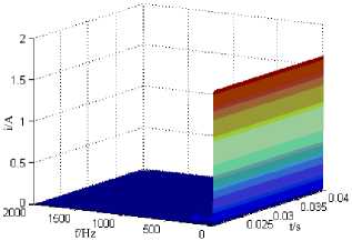
(g) Hilbert amplitude spectrum at 5000 ^Ω

14 ----------------------.-----------------------.-----------------------.----------------------

1 2                                                                               -

1                                                                                                                -

08                                                  -

0.8

04                                                  -

0.2

О *-------------------------------------------------

О          500         1000        1500        2000

f/Hz

• (h) Hilbert marginal spectrum at 5000 ^Ω

Fig.10. The influence of the grounding resistance on the transient timefrequency characteristics of fault line zero sequence current

In short, with the continuous increase of the grounding resistance, the system undergoes a sate of less damping, over damping, and then to less damping, the signal is towards the low frequency in general, the frequency components are more and more concentrated, and the energy distribution is becoming more and more concentrated.

• V. C ONCLUSION

In this paper, the transient analysis of single-phase grounding current in small current grounding power grid is carried out. Resultly the grounding current is mainly capacitive current and inductance current. On this basis, the theoretical analysis and simulation are done. According to the different fault conditions, such as feeder structure, fault phase, grounding resistance, fault distance, etc, the simulation results show that the fault phase and the grounding resistance have most influence on the feeder zero sequence current.

The main results of this paper are as follows:

• (1)    Analyze the steady-state and transient characteristics of single phase grounding fault in the small current grounding power grid, in which the neutral point is not connected to ground or connected to ground through the arc suppression coil.

• (2)    Under the EMTP_ATP environment, a small current grounding system is built, and the simulation analysis of the single-phase grounding fault under different conditions is done. According to the power system related theory calculation result, the system grounding capacitance over 10KV voltage level is allowed the maximum capacitance current 20A, the neutral point must be connected with the arc suppression coil, and the compensation degree is 10%.

• (3)    HHT is applied to the single phase grounding fault detection through the arc suppression coil. Firstly, a time window is selected to extract the transient component of the fault signal, and the transient component of the feeder zero sequence current is extracted, and the time frequency analysis of transient signal is done with the HHT. The two main factors that influence the transient signal, the fault phase and the grounding resistance, are studied respectively.

A CKNOWLEDGMENT

The authors wish to thank my graduate tutor Hongbin Wu Professor and Benxian Xiao Professor and graduate student Lin Zhang.