
Choice of a method for assessing the depth of the tempered layer in a martensitic steel welded joint
Журнал: Nanotechnologies in Construction: A Scientific Internet-Journal @nanobuild-en
Рубрика: System solutions for technological problems
Статья в выпуске: 5 Vol.18, 2026 года.
Бесплатный доступ
Introduction. This review considers the choice of a nondestructive testing method for estimating the depth of the tempered martensitic layer in welded joints of martensitic steel pipes after high-temperature tempering. During heat treatment of welded joints, martensite does not always decompose through the entire weld thickness, especially in the root zone of thick-walled pipes, and averaged characteristics may conceal local areas of increased hardness and brittleness. Methods and Materials. Four groups of methods were compared: eddy current testing, magnetic Barkhausen noise analysis, ultrasonic methods and magnetic coercimetry. For each group, the depth from which the signal carries information about the structural-phase state and nanoscale features of the weld metal was assessed. Results. Eddy current and Barkhausen methods mainly characterize the surface and near-surface layer. Ultrasonic methods can probe deeper layers, but when the acoustic contrast between structures is weak, the tempered-layer boundary is difficult to identify from the backscattered signal, and the results are difficult to interpret. Coercimetry was chosen for field conditions. Interchangeable attached U-shaped electromagnets of different sizes magnetize the metal to different depths, which makes it possible to construct a conditional layer-by-layer magnetic profile. Discussion. It is proposed to select transducers, construct calibration curves on welded specimens, and check the transformed-layer thickness estimate by metallography, microhardness testing and, if necessary, X-ray diffraction. Conclusion. The resulting layer-by-layer profile is conditional. Depth estimation requires calibration for the specific steel grade and welding technology, with allowance for residual stresses and transducer orientation. Pipe inspection also requires allowance for lift-off, surface curvature and weld reinforcement.
Короткий адрес: https://sciup.org/142249023
IDS: 142249023 | DOI: 10.15828/2075-8545-2026-18-5-691-700
Текст научной статьи Choice of a method for assessing the depth of the tempered layer in a martensitic steel welded joint
Review article
Файрушин А.М., Туманова Е.Ю., Собачкин А.С., Имаев М.Ф., Токарев А.С., Мусина Д.Р. Выбор методики оценки глубины отпущенного слоя сварного шва мартенситной стали. Нанотехнологии в строительстве. 2026;18(5):691–700. https://doi. org/10.15828/2075-8545-2026-18-5-691-700. – EDN: CQGODM.
Martensitic-grade steel pipes are widely used in the oil and gas industry. Domestically produced pipes range from 11 to 550 mm in diameter, while wall thicknesses range from 1.5 to 40 mm depending on the forming process (cold or hot) and the applicable standard [1]. Pipes of this class – most commonly grades 15Kh5M, 20Kh13, 15Kh11MF, and 12Kh11V2MF – are manufactured by a seamless process and used under severe service conditions in petroleum refining (cracking furnace tubes), the chemical industry, and well construction involving highly corrosive fluids [1, 2, 3]. During cooling after fusion welding, a martensitic structure forms in the weld metal. Because martensite is brittle, high-temperature tempering is required to decompose it into ferrite and cementite. Tempering is generally performed using surfacemounted electric heaters. However, martensite does not always decompose through the full weld depth; it often remains in the weld root, especially in thick-walled pipes. Selecting a nondestructive testing (NDT) method for assessing the extent of martensite decomposition is therefore important. A characteristic averaged over the weld depth is insufficient because the transformation depth must also be estimated. An averaged characteristic does not reveal the distribution of tempering through the depth and may conceal local areas of untempered martensite. A thin layer of untempered or insufficiently tempered martensite may contribute little to the average value, so a welded joint may meet the acceptance criterion based on the average value even though a locally harder and more brittle zone remains at the surface, the fusion line, the weld root, or in the heat-affected zone (HAZ), where it acts as a stress concentrator. Tempering changes martensite lattice te-tragonality, the dislocation structure, and carbide dispersion. These changes affect the coercive force [17–19], so magnetic measurements provide indirect information about the structural state of the metal. Their individual contributions cannot be separated using a single magnetic parameter.
The aim of this work is to select an NDT method suitable for field assessment of the heat-treatment quality of martensitic-grade steel pipe welds, including evaluation of the completeness of martensite decomposition through the wall thickness of the welded joint.
METHODS AND MATERIALS
The NDT methods applicable to this task are considered below (Table 1). Eddy current testing is sensitive to changes in electrical conductivity and magnetic permeability and can therefore respond to structural heterogene-
Nanotechnologies in construction
Нанотехнологии в строительстве
2026; 18 (5): 691–700
SYSTEM SOLUTIONS FOR TECHNOLOGICAL PROBLEMS
Nanob
Table 1. Effectiveness of NDT methods for assessing the completeness of tempering through the welded-joint cross-section
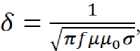
where δ is the penetration depth (skin depth); f is the alternating-current frequency; µ0 is the permeability of free space; µ is the magnetic permeability of the medium; σ is electrical conductivity.
In ferromagnetic steel, high µ sharply reduces δ; at megahertz frequencies, the penetration depth is therefore a fraction of a millimeter [5]. Millimeter-scale depths require low frequencies, multifrequency or pulsed configurations, control of sensor-to-metal lift-off, and calibration using specimens of the same steel and geometry [4]. Eddy current testing is consequently suitable as a surface and near-surface indicator [6]. Estimating the tempered-zone depth in a weld quantitatively with this method is difficult, because the instrument must be precisely calibrated for the specific microstructure and lift-off variations on the uneven weld bead must be taken into account [7].
The magnetic Barkhausen noise method is based on detecting jumps of domain walls pinned by dislocations, secondary-phase particles, grain boundaries, and residual stresses. It is used for mapping near-surface tempering, residual stresses, and structural heterogeneity [8]. The signal formation depth is small and, in hard, fine-grained structures, including martensitic ones, amounts to tens or hundreds of micrometers [9]. The thickness of hardened layers in the millimeter range was estimated indirectly, using models built on specimens that relate near-surface signal parameters to hardening depth [10, 11]. In the present task, the method is suitable for preliminary testing of the weld surface but does not measure the tempered-layer depth directly.
Ultrasonic methods can probe metal to a depth of several millimeters. In [12, 13], the depth of hardened and carburized layers was determined from the back-scattered signal of shear waves introduced at an angle to the surface. For welded joints of martensitic chromium steels after heat treatment, tomograms (maps of elastic-wave velocity) have also been constructed [14]. Boundary detection from the backscattered signal has been described for induction-hardened parts, where the structure changes sharply at the edge of the hardened layer [15]. In a tempered weld, the transition between the martensitic and partially tempered (sorbitic) structures may be gradual, and if the weld metal and HAZ are nearly homogeneous through the wall thickness, the boundary is difficult to identify from this signal. Instead, the phase or group velocity of the waves and their attenuation or scattering are mapped [16], and the resulting maps are compared with metallography and microhardness measurements.
Magnetic coercimetry, based on measurement of the coercive force (Hc), was selected for further analysis because the depth of the tested zone can be changed by selecting the dimensions of the attached electromagnetic transducer. The method is applicable to ferromagnetic steels and allows the magnetic properties of individual regions of a welded joint to be assessed. The Barkhausen noise signal is formed by weak high-frequency electromagnetic pulses that attenuate in the metal at depths of
Nanotechnologies in construction
Нанотехнологии в строительстве
2026; 18 (5): 691–700
Nanob
SYSTEM SOLUTIONS FOR TECHNOLOGICAL PROBLEMS
fractions of a millimeter. Under quasistatic magnetization reversal in coercimetry, the testing depth is governed mainly by transducer geometry and magnetic circuit reluctance.
RESULTS
Coercive force is a structure-sensitive parameter of ferromagnetic steels. It increases with the density of fine structural defects and dislocations, the total extent of grain boundaries, and internal stresses that act as effective obstacles to domain-wall motion. During high-temperature tempering, the supersaturated solid solution decomposes, martensite lattice tetragonality decreases, carbon redistributes, nanoscale carbides precipitate and coarsen, and microstresses relax. In most cases, these processes reduce magnetic hardness relative to the freshly quenched or undertempered condition. Hc measurements have therefore long been used to monitor the quality of thermal and thermochemical treatment of steel products [17, 18, 19].
The basic principle for measuring Hc in extended products is local magnetization to saturation using an attached U-shaped electromagnet [17, 20] (Fig. 1). An attached electromagnet made of a soft-magnetic material magnetizes a local region, rather than the entire object, to a specified depth below the surface. From the depth distribution of magnetic induction in a massive plate, Mikheev [17] concluded that when the pole width bp equals the width of the magnetized plate, the magnetization depth zp of a U-shaped electromagnet with a pole thickness-to-width ratio ap:bp = 1:3 is approximately equal to the pole thickness. As the plate surface area increases, zp may decrease to 0.5ap because of lateral magnetic-flux leakage.
Reference [21] summarizes Hc measurements of massive products using attached two-pole electromagnets of different geometries. It shows that the minimum thickness hm of a homogeneous massive body, above which a further increase in thickness has almost no effect on the coercimeter reading, is approximately proportional to the square root of the pole area:
h m = 2√S e . (2)
This means that the magnetic properties of layers located deeper than hm have almost no effect on the measured demagnetizing current. The value hm can therefore be regarded as the maximum depth from which a given attached electromagnet can obtain information about material structure.
For a surface-hardened layer, a maximum measurable thickness hk was also introduced. Up to hk, the coercimeter reading depends appreciably on layer thickness, which allows this range to be used for quantitative estimation of hardened-layer depth:
hk ≈ 0.6√Se. (3)
When the layer thickness exceeds hk, the increase in the reading slows, and the instrument increasingly characterizes the layer’s own coercive force rather than its thickness. For an electromagnet with a pole width-to-thickness ratio b/a ≈ 3, hk is close to the pole thickness a, consistent with earlier recommendations for selecting the geometry of attached electromagnets [17].
An initial thickness hn was also defined; a thinner layer has almost no effect on the coercimeter reading [21]:
hn ≈ 0.03√Se. (4)
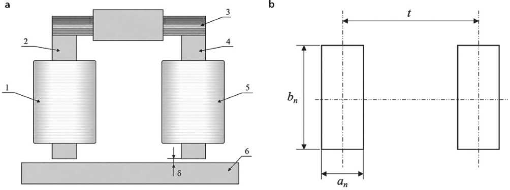
Fig. 1. (a) Schematic of an attached U-shaped electromagnet on the test object: 1, 5 – magnetizing (demagnetizing) coils; 2, 4 – core elements; 3 – magnetic-field sensor (ferroprobe); 6 – test object; δ – lift-off gap. (b) Diagram of a rectangular electromagnet, where ap, bp, and t are pole thickness, pole width, and interpole distance, respectively [19, 20]
Nanotechnologies in construction
Нанотехнологии в строительстве
2026; 18 (5): 691–700
Nanob
SYSTEM SOLUTIONS FOR TECHNOLOGICAL PROBLEMS

The given electromagnet does not reliably measure the thickness of such a layer, and the reading depends mainly on the properties of the substrate or core.
The three boundaries hn, hk, and hm divide the generalized curve reported in [21] into four regions (Fig. 2). Thickness is measured in region II between hn and hk, where the readings depend simultaneously on the coercive force of the magnetically hard layer, its thickness, and the properties of the core. In region I (h < hn), the readings are determined mainly by the core. In region III (hk < h < hm), the effect of layer thickness weakens, and in region IV (h > hm) the readings correspond to a homogeneous massive product. Knowing these boundaries, one can select the pole area for the expected layer thickness or, conversely, evaluate the capabilities of an existing electromagnet with a known Se.
For a correct Hc measurement, the object must be magnetized to a level close to technical saturation. Modeling has shown that preliminary magnetization of the test region to near technical saturation is achieved when the cross-sectional area of the test region is smaller than or comparable to the cross-sectional area of the electromagnet poles and any lift-off gaps between the transducer and the object are sufficiently small. When magnetizing massive objects, the interpole distance should be reduced by using converging pole pieces to obtain the required magnetic-flux density [22].
An attached electromagnet does not measure Hc directly. The instrument measures a demagnetizing current Ic that is related to Hc. For a U-shaped attached transducer with a built-in zero magnetic-flux indicator, reference [23] expresses the relationship between the demagnetizing current Ic and the coercive force Hc of a homogeneous magnetized volume as:
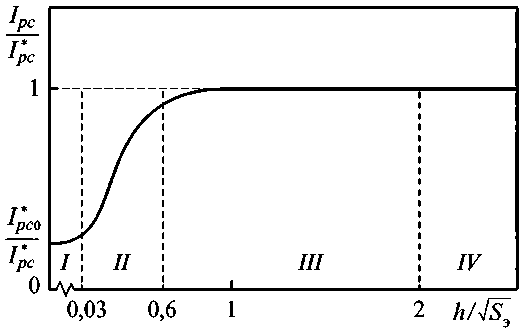
Fig. 2. Generalized coercimeter response curve in relative units. Ordinate notation: Ipc – demagnetizing current; I*pc – demagnetizing current of a structurally homogeneous massive product with thickness h ≥ hm; I*pc0 – demagnetizing current of the soft-magnetic core [2p1]
1 Г ^Fl ^cu
W i-Rp^+Rg+Rn
+ ^ce
where W is the total number of turns in the electromagnet winding; Ucu is the magnetic-potential drop across the test object; Uce is the magnetic-potential drop across the electromagnet; RF1 is the reluctance of the flux path through air between the poles; Rδ is the reluctance of the lift-off gaps between the poles and the object; and Ru is the reluctance of the test object.
Because Ucu is related to Hc and to the length of the magnetic field line in the object, the expression shows that the demagnetizing current depends not only on metal properties but also on object geometry, lift-off, and circuit reluctance. For a welded joint, the instrument reading therefore requires calibration and characterizes the magnetized volume as a whole rather than the intrinsic Hc of an individual microregion.
Approximate Hc values for the steels of interest in different structural states are useful when selecting measurement equipment and planning experiments. For the widely used 15Kh5M steel, these data were not found together in a single publication. Reference [24] reports Hc = 6–7 A/cm for 15Kh5M furnace coils after long-term service. T91/P91 steel, an analogue of 15Kh5M, has Hc = 19.65–20.47 A/cm in the as-welded condition, whereas after prolonged tempering it does not exceed 10.75 A/cm [25]. Published Hc values can be used only as reference points, and acceptance testing of a welded joint requires a dedicated calibration.
Basic Methodological Framework
In surface-hardened products, the hardened layer follows the product surface. A weld is oriented differently: its plane runs across the product surface. The welded joint is also structurally heterogeneous. Moving outward from the weld metal, the weld (solidification) zone, the fusion zone (the boundary between weld metal and base metal), and the HAZ occur in sequence. The model of a surface layer over a substrate therefore applies only partially to a welded joint. In thick-walled products, it is difficult to measure the coercive force of the weld metal separately from the contributions of the HAZ and base metal, even when the electromagnet pole width is comparable to the weld width. In practice, an attached electromagnet averages the response of the weld, the HAZ, and part of the base metal. If the weld is sufficiently wide and the wall is thin, however, the attached electromagnet can be oriented along the weld. This orientation reduces the influence of the fusion zones and HAZ, allowing the depth profile of the weld metal itself to be estimated [26, 27].
After high-temperature tempering of a martensitic steel weld, the surface layer of the joint consists of tempered or decomposed martensite and has a lower Hc than
Nanotechnologies in construction
Нанотехнологии в строительстве
2026; 18 (5): 691–700
Nanob
SYSTEM SOLUTIONS FOR TECHNOLOGICAL PROBLEMS
the martensitic core. The initial values of the generalized curve will therefore exceed unity (Fig. 3), where I*pc is the demagnetizing current of a structurally homogeneous massive product with a soft-magnetic structure and thickness h ≥ hm, and I*pc0 is the demagnetizing current of the magnetically hard core. In region I (0 to hn ≈ 0.03√Se), corresponding to electromagnets with large pole crosssections, coercimeter readings are almost constant and depend mainly on the coercive force of the martensitic core. In region II (hn to hk ≈ 0.6√Se), corresponding to a medium-sized electromagnet, the readings depend on the coercive force and thickness of the tempered layer and on the coercive force of the martensitic core. In region III (hk to hm = 2√Se), corresponding to an electromagnet with a still smaller cross-section, the readings are governed mainly by the coercive force of the tempered layer and depend only weakly on changes in its thickness and the properties of the martensitic core. In region IV (h ≥ hm), corresponding to electromagnets with the smallest crosssections, the readings depend only on the coercive force of the tempered layer.
Procedure for Measuring Transformed-Layer Thickness
-
1. Prepare the test area: remove scale and contaminants, ensure repeatable pole contact, specify the permissible lift-off, use radius-matched tooling for the pipe, and define the orientation of the U-shaped electromagnet relative to the weld.
-
2. For each interchangeable electromagnet, determine Se = a × b and calculate hn ≈ 0.03√Se, hk ≈ 0.6√Se, and hm ≈ 2√Se. Select a set of transducers such that the expected transformed-layer thickness lies within the working interval hn< h < hk for at least one transducer.
-
3. Prepare calibration specimens made from the same steel and welded joint: specimens in the as-welded condition without tempering, after the standard high-temperature tempering cycle, and after cycles that produce different depths of transformed or undertempered material.
-
4. Select the criterion that defines the transformed-layer boundary and measure its depth on metallographic sections. Examine the micro- and nanostructure and the microhardness distribution through the weld depth and, if necessary, assess the degree of martensite decomposition by X-ray diffraction.
-
5. For each selected electromagnet, use the calibration specimens to construct an Ipc(h) or Hc(h) relationship, preferably in normalized form as a function of h/√Se. Because the tempered layer is magnetically softer than undertempered martensite, the calibration curve will have the reverse trend (Fig. 3), but the working boundaries hn, hk, and hm retain their meaning.
-
6. On the test object, perform a series of measurements at the same weld locations. First demagnetize the region or stabilize its magnetic state, install the transducer, magnetize to near technical saturation, and record the demagnetizing current Ipc or the calculated Hc. Make at least three repeated measurements at each point and discard readings associated with an evident loss of contact.
-
7. Use the calibration curve to find the normalized thickness x = h/√Se and calculate h = x√Se. An estimate obtained within hn< h < hk is considered quantitative. Values below hn indicate a layer thinner than the lower sensitivity limit of that electromagnet; values above hk provide only a lower bound for thickness or indicate that a larger transducer is required.
-
8. Reconcile the results obtained with several electromagnets. If the readings of the small transducer have already reached the plateau of the calibration curve (h > hk) while the medium transducer remains within its working interval, determine the depth from the medium transducer. If the readings of all transducers are on the plateau, report h ≥ hk for the largest working transducer and, if necessary, use an electromagnet with a larger Se. If only the small transducer detects a deviation, classify the layer as surface or near-surface.
-
9. In the test report, state not only the estimated thickness h but also the pole dimensions and orientation, lift-off, surface curvature, weld-reinforcement height, number of repeats, scatter of the readings, and the criterion used to correlate the magnetic boundary with the transformation boundary determined by metallography or microhardness.
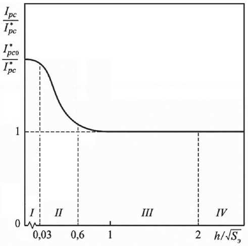
Fig. 3. Expected generalized coercimeter response curve in relative units for a product with a soft-magnetic surface layer and a magnetically hard core
Nanotechnologies in construction
Нанотехнологии в строительстве
2026; 18 (5): 691–700
Nanob
SYSTEM SOLUTIONS FOR TECHNOLOGICAL PROBLEMS
Instruments for Method Implementation
A single fixed attached electromagnet cannot cover the full practically significant range of pipe wall thicknesses. An instrument system is therefore used, comprising a magnetic structure analyzer or coercimeter with a set of interchangeable U-shaped transducers and pole pieces. Traditionally, such tasks were addressed using KIFM-1 and KF-1 coercimeters and their modifications [18, 19, 28, 29]. Multiparameter systems are also used that are capable of measuring not only coercive force but also residual flux, maximum magnetic flux, or the tangential field within a single cycle. Reference [30] demonstrates the capabilities of the SM-401 magnetic structure analyzer with an attached electromagnet for monitoring quenching and tempering. Reference [23] shows the advantages of measuring Hcby the internal field, and in [31] Hc was used together with magnetic flux to selectively estimate layer thickness and degree of hardening.
Interchangeable pole pieces are required in three cases. First, when pipes of different diameters are tested, flat poles produce variable lift-off on a curved surface; quantitative measurements therefore require pole pieces matched to the outside radius. Second, narrow pole pieces are used for testing a narrow weld or fusion line to reduce the influence of the HAZ and base metal. Third, thick welds require poles with a larger cross-section, because the contribution of the deep region to the reading of a small transducer is small and the testing depth increases with the pole cross-sectional area (Eqs. 2–4). Calibration is valid only for the pole-piece configuration with which it was performed. Pole geometry changes circuit reluctance and flux distribution and, with them, the depth of the region contributing to the reading.
DISCUSSION
Calibration, Errors and Limitations
The tempered-layer thickness can be estimated quantitatively only after calibration on welded specimens of the same steel, with a similar thickness and made using the same welding procedure. Criteria obtained for P91, 30KhGSA, or carburized layers can be used only as a physical reference for 15Kh5M steel. We propose including specimens in the as-welded condition without tempering, after the standard high-temperature tempering cycle, and after undertempering. Tempering time, temperature, or heating power is varied to obtain specimens with different structural distributions through the depth. Each specimen is first measured with all transducers and then sectioned for metallography and microhardness measurements. Changing the tempering cycle affects both the layer depth and the degree of tempering within the layer. To establish the relationship between instrument readings and layer thickness, specimens with similar layer and core structures and microhardness values are therefore compared. If this similarity has not been confirmed, a relationship based on thickness alone is insufficient: the calibration model must account for differences in structural state. The tempered-layer boundary is defined by the chosen metallographic or microhardness criterion. The magnetically altered zone is compared with this boundary on the calibration specimens; their depths are not assumed to coincide.
The magnetic measurements are compared with the results of macrosection and microsection examination. The HAZ width and structure are determined on these sections. Microhardness is measured along profiles from the surface and from the weld axis. X-ray diffraction is used to refine the phase composition. The tetragonality of martensite is estimated from the splitting of diffraction peaks. At the low tetragonality typical of low-carbon and tempered martensite, the peak splitting may not be resolved. The following relation is used:
1 _ h2+k2 I2
, ahkl a c where dhkl is the interplanar spacing for the reflection with indices hkl and a and c are the tetragonal lattice parameters of martensite. A decrease in the c/a ratio during tempering is one indicator of martensite decomposition, but for a welded joint this criterion must be compared with microhardness and microstructural analysis.
A significant error is introduced by the lift-off gap between the poles and the product. It increases circuit reluctance and lowers the coercimeter reading [22]. A 1 mm lift-off reduced KIFM-1 readings by more than 33%, whereas the readings of MMT-3, which operates using the internal field, decreased by less than 9% [23]. Lift-off effects can be reduced by accounting for additional magnetic parameters and measuring the tangential field component [32, 33]. The symmetry of the measured field also depends on the positions of the field and flux sensors in the transducer [34]. On a pipe, surface curvature and weld reinforcement add to the lift-off. The procedure specifies the permissible lift-off and reinforcement height in advance. It defines surface preparation, magnet orientation, and the demagnetization sequence. The number of repeated measurements and the outlier-rejection rule are fixed before testing. Residual stresses and residual magnetization affect the readings as well. The stress and structural contributions cannot be separated from a single Hc measurement. Because high-temperature tempering both relieves stresses and changes the structure, it is validated on a calibration series whose stress state is close to that of the actual product. Without such validation, the detected magnetic heterogeneity cannot be unambiguously related to the depth of the tempered layer.
Nanotechnologies in construction
Нанотехнологии в строительстве
2026; 18 (5): 691–700
Nanob
SYSTEM SOLUTIONS FOR TECHNOLOGICAL PROBLEMS
Method Limitations
The instrument averages the response over the entire volume through which the magnetic flux closes. For this reason, the layer-by-layer profile obtained with a set of electromagnets is conditional. It does not resolve adjacent layers in a narrow HAZ. Different transducers sample non-coincident volumes of metal. Magnetic anisotropy due to directional solidification of the weld and precipitation of dispersed carbides during tempering influence the readings as well. Calibration is performed on welded specimens for each steel grade. A calibration relationship from another grade may be used if testing on specimens of the steel under examination confirms that the thickness estimates meet the error limit specified in the procedure. Otherwise, a new calibration relationship is established. CONCLUSION
Of the NDT methods considered, magnetic coercim-etry with a set of interchangeable attached transducers was selected for estimating the depth of the tempered layer in welds of martensitic steels. After calibration, a single attached electromagnet gives an integral estimate of Hc over the magnetized volume. A set of electromagnets with different cross-sections provides a conditional layer-bylayer profile. A small electromagnet characterizes the surface layer, the reading of a medium one also includes the transition region, and a large one covers a deeper volume of the joint. The diagnostic feature is the change in Hc with increasing magnetization depth, since the absolute Hc value also depends on the degree of tempering and the properties of the core. The result is verified by metallography, microhardness testing, and, if necessary, X-ray diffraction analysis of martensite tetragonality and its nanoscale features. Further verification of the procedure should assess how much the simultaneous measurement of Hc, residual and maximum magnetic flux in the transducer-object circuit [32], and the tangential field between the poles reduces the ambiguity in separating the effects of layer depth and degree of tempering.