Classification of ECG Using Chaotic Models

Central tendency measure (CTM) has also become very useful in describing the chaotic behavior of the system. When used with clinical parameters [1], CTM can become a powerful indicator of the absence of congestive heart failure. The CTM method for determining variability in nonlinear time series has been shown to be effective in both time series with inherent patterns, such as ECGs and in timer series without a pattern such as hemodynamic studies [2]. CTM can be used along with other techniques like CD, and ApEn to study the underlying chaos in the ECG [3, 4, 5].

The phase space of a dynamical system is a mathematical space with orthogonal coordinate directions representing each of the vectors needed to specify the instantaneous state of the system. Usually taken method of delays is used to construct an attractor of dynamical system in a multidimensional state space from only the knowledge of a one-dimensional time sequence that describes the system behavior [6, 7].

Studies have been performed to obtain the phase space density plot by mapping the distribution of points in the phase space of ECG signals and the phase space density values within a predefined window were used for arrhythmia detection [8]. Classification was performed using a multilayer back propagation neural network and very good result was obtained for classifying cardiac arrhythmias like premature ventricular contraction, atrial fibrillation, ventricular tachycardia and ventricular fibrillation. Phase space portrait of a single cycle ECG wave has also been derived to study the chaos of the system [9]. The aim of this work is to use the chaotic model to analyze and define the arrhythmia that may be observed in an ECG signal. Chaos may be defined as the pattern that lies between the determinism and randomness of a system. Normally Chaos is analyzed using phase space portrait and central tendency measure. These non-linear techniques are applied on the bit-to-bit interval (BBI) and instantaneous heart rate (IHR) that are derived from the sample ECG records from MIT-BIH database [10]. The results found from this work are analyzed to see if there is any abnormality present in the examined ECG record.

• II.    Review of Some Ecg Analysis Techniques

A large variety of techniques for ECG analysis have been proposed and published over the last two decades. These techniques have become essential in a large variety of applications, from diagnosis through supervision and monitoring applications. In general, ECG analysis techniques may be divided into two broad categories: conventional (manual) method and the automated method. Classical techniques have been used to address this problem such as the analysis of electrocardiogram (ECG) signals for arrhythmia detection using the frequency domain features, using time domain analysis, and wavelet transform. Other techniques used adaptive filtering, sequential hypothesis testing. Recently, there has been an increasing interest in applying techniques from the domains of nonlinear analysis and chaos theory in studying biological systems. The objective of this chapter is to present some of the techniques for ECG signal analysis.

• A.    Frequency domain analysis

In the frequency domain analysis approach of ECG, first the data set is determined from the QRS complex in the ECG signal. Then the QRS complexes are used for Fast Fourier Transform (FFT), from which the power spectrum is calculated. Before computing the Fourier transform, a window (e.g., Hanning window) is applied to completely suppress the discontinuities due to adjacent T-wave and P-wave.

• B.    Time domain analysis

Time domain analysis of ECG is usually simpler and produces results in real time. The two most common parameters for estimating heart rate variability in the time domain are: SDNN and RMSSD. They are both expressed in milliseconds [1, 2]. SDNN is the standard deviation of the normal-to-normal R-peak intervals and provides a measure of the total variability. RMSSD is the root mean square of successive differences. This last parameter quantifies the standard deviation of the differences between neighboring intervals and estimates the parasympathetic drive of the autonomic nervous system [11].

• C.    Wavelet transform

The wavelet transform has been used in the biomedical signal processing and has an important role in the ECG characterization and QRS detection. These class of algorithms for ECG signal processing normally uses discrete wavelet transforms (DWT), dyadic wavelet transform (DyWT) and continuous wavelet transforms (CWT), and all of them with real wavelet functions to decompose, analyze, and compress the ECG signals [12].

The Fourier Transform (FT) decomposes signals in infinite extended sinusoidal functions, requiring the stationary hypothesis; so all the information localized in time, such QRS complex, is spread over the entire frequency axis. The Short Time Fourier Transform (STFT) is useful if the signal is non-stationary over the whole interval, but maintains its frequency characteristic during the short time interval [13]. The STFT provides time-frequency information: a local spectrum is performed by windowing the signal through fixed dimension windows where it may be considered approximately stationary. The window dimension fixes both time and frequency resolutions. The Wavelet Transform (WT) is a tool for non-stationary signal processing that is alternative both to the classical spectral analysis in the frequency domain and to the STFT. The WT overcomes the fixed resolution analysis of the STFT. It satisfies the uncertainty principle or Heisenberg inequality, so time resolution increasing lowers frequency resolution.

• D.    Non-linear techniques

Poincare plots have been used to track the stability of nonlinear systems. A Poincare plot is obtained for a time sequence where the value at time n is represented by a by plotting a vs. a . The resulting plot is a measure of the degree of stability in the system. These plots lie in the first quadrant. An example is given is Fig. 1. This problem have been approached from another viewpoint, and been developed to second-order difference graphs, which consist of the plot: d2 = (a n+2 – a n+1 ) vs. d1 = (a n+1 - a n ) for all values of n. These plots are centered around the origin and are useful in modeling biological systems, such as hemodynamics and heart rate variations . The second order-difference approach gives a picture of the rate of change of the stability of the system [6, 7]. Fig. 2 shows the second-order difference plot which is analogous to Fig. 1.

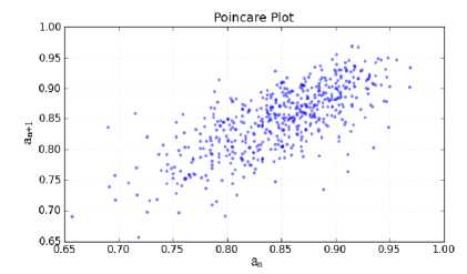
Figure 1: Poincare plot.

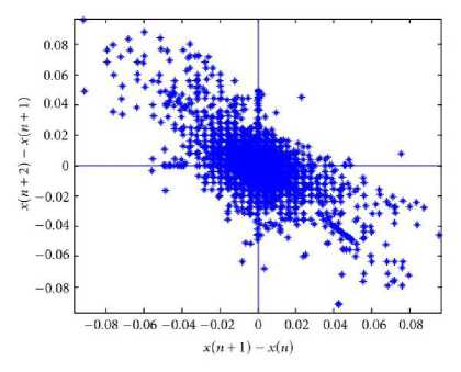
Figure 2: Second order difference plot.

The measure of central tendency of the second-order difference plots provides useful summary. It is computed by selecting a circular region around the origin of radius r, counting the number of points which fall within the radius, and dividing by the total number of points. Let t = total number of points, and r = radius of central area. Then, t - 2

n = [E ^( diM1 — 2)                     (1)

i = 1

Where, ^(d ) = 1

If,

^[( a i + 2 ^{- a}i + 1^{)2 + ( a}i + 1 ^- a i ⁾² ] ^0.5 <  r               ⁽²⁾

= 0 otherwise

Here for applying the CTM, we used the data set obtained from bit-to-bit interval and the instantaneous heart rate. It is observed that for a healthy person, data set tends to be confined in a small area and hence the CTM tends to be high. For ailing person, the data set tends to be dispersed in a broader area and hence the CTM tends to be low.

• E.    Standard Deviation

In probability and statistics, the standard deviation of a probability distribution, random variable, or population or multi-set of values is a measure of the spread of its values. It is usually denoted with the letter σ (sigma). It is defined as the square root of the variance. To understand standard deviation, it should be kept in mind that variance is the average of the squared differences between data points and the mean. Variance is tabulated in units squared. Standard deviation, being the square root of that quantity, therefore measures the spread of data about the mean, measured in the same units as the data. Said more formally, the standard deviation is the root mean square (RMS) deviation of values from their arithmetic mean. The standard deviation is the most common measure of statistical dispersion, measuring how widely spread the values in a data set is. If the data points are close to the mean, then the standard deviation is small. As well, if many data points are far from the mean, then the standard deviation is large. If all the data values are equal, then the standard deviation is zero [1].

• F.    Coefficient of variation

Coefficient of variation (CV) is a measure of dispersion of a probability distribution. It is defined as the ratio of a standard deviation σ to the mean μ.

Cv = -                                 (3)

Ц

The coefficient of variation is a dimensionless number. For distributions of positive-valued random variables, it allows comparison of the variation of populations that have significantly different mean values. It is often reported as a percentage (%) by multiplying the above calculation by 100. When the mean value is near zero, the coefficient of variation is sensitive to change in the standard deviation, limiting its usefulness.

• G.    Phase space portrait

  A phase space, introduced by Willard Gibbs in 1901, is a space in which all possible states of a system are represented, with each possible state of the system corresponding to one unique point in the phase space. In order to reconstruct the phase space using a time series, it is resolved into coordinate values of a d dimensional embedding space by one of the known embedding methods. The most frequently embedding method is the time delay embedding in which delayed values of the time series are used to obtain the reconstructed vectors:

x[n]=[x[n], x[n-τ], x[n-2τ], ……, x[n-(d-1)τ] ] (4)

Here τ is the delay time and d is the embedding dimension. If the time series has N elements, the number of reconstruction vectors will be N-(d-1)τ. It should be noted that if d is high enough the reconstructed phase space portrait gives the phase portrait of the real system.

• H.    Lyapunov Exponents

Lyapunov exponent is simply a measure of how fast two initially nearby points on a trajectory will diverge from each other as the system evolves, thus giving information about the system’s dependence on initial conditions. A positive Lyapunov exponent is a strong indicator of chaos. Even though an m dimensional system has m Lyapunov exponents, in most applications it is sufficient to compose only largest Lyapunov exponent (LLE). The average largest Lyapunov exponent is calculated as follows. First, a starting point is selected in the reconstructed phase space and all the points which are closer to this point than a predetermined distance, ε, are found. Then the average value of the distances between the trajectory of the initial point and the trajectories of the neighboring points are calculated as the system evolves. The slope of the line obtained by plotting the logarithms of these average values versus time gives the LLE. To remove the dependence of calculated values on the starting point, the procedure is repeated for different starting points and the average is taken as the average LLE [14, 15].

• III.    Proposed Method

This work presents heart rate variability (HRV) analysis using some non-linear methods. The ECG signal to be analyzed is first processed [16] to extract the QRS complex. From that bit-to-bit interval (BBI) is calculated. From the BBI we get the instantaneous heart rate (IHR). On this dataset of BBI and IHR, various non-linear parameters like standard deviation (SD), coefficient of variation (CoV), central tendency measure (CTM), phase space portrait are determined. The result obtained from the application of these non-linear techniques is analyzed to distinguish the ECG signals between the healthy person and that of the ailing person. The ECG signals on which the proposed non-linear methods are applied for analysis are taken from the MIT-BIH Arrhythmia Database [10], where the sampling rate is 360 Hz and sample resolution is 11 bits/sample [1, 2, 5].

• IV.    Analyzing Steps

At first, the ECG signal obtained from MIT-BIH database [10] is partitioned into its periods or beats. A beat is defined as the signal between two R waves as ECG signal is quasi periodic, the lengths of the partitioned blocks (beats) are not equal. Hence the Bit-to-Bit Interval (BBI) is obtained which is the instantaneous distance between two adjacent R waves. BBI is measured in seconds. From BBI, Instantaneous Heart Rate (IHR) is calculated using the following formula:

IHR =

BBI

IHR is measured in the unit bits per minute (bpm).

Thus two data sets are obtained. One comprises the BBI and the other consists of IHR. On these two data sets the following non-linear methods are applied to analyze the chaotic behavior of the ECG.

• A.    Standard Deviation

In probability and statistics, the standard deviation of a probability distribution, random variable, or population or multiset of values is a measure of the spread of its values. It is usually denoted with the letter σ (sigma). It is defined as the square root of the variance.

Said more formally, the standard deviation is the root mean square (RMS) deviation of values from their arithmetic mean. The standard deviation is the most common measure of statistical dispersion, measuring how widely spread the values in a data sets are. If the data points are close to the mean, then the standard deviation is small. As well, if many data points are far from the mean, then the standard deviation is large. If all the data values are equal, then the standard deviation is zero. Following equation describes the standard deviation used in this project:

5 =

n

1 E x-n -=1 к

x

к

Where, x =

n

1E x- n i=1

And n is the number of elements in the data set.

• B.    Coefficient of Variation

Coefficient of variation is a statistical measure of the dispersion of data points in a data series around the mean. It is calculated as follows:

Coefficient of variation = Standard deviation / Mean (7)

• C.    Central Tendency Measure

Central tendency measure (CTM) is used to quantify the degree of variability in the second order difference plot. It is calculated by selecting a circular region of radius r, around the origin, counting the number of points that fall within the radius, and dividing by the total number of points. If t = total number of points, and r = radius of central area. Then, t-2

n = E 5(d-^]/( t - 2)                       (8)

i = 1

Where, ^(d;) = 1

If,

^[( a - + 2 ^- a - + 1 ) 2 ^{+ (} a - + 1 ^- a - ⁾² ] ^0.5 <  r               ⁽⁹⁾

= 0 otherwise

In our project, the data set from BBI and IHR are used to measure the CTM. In first step, the optimum radius is determined for the circular region. For that, the statistical technique analysis of variance (ANOVA) is used [17]. In this project the one-way ANOVA, is used for comparing the means of two or more columns of data in the m-by-n matrix X, where each column represents an independent sample containing m mutually independent observations. Using the ANOVA f-value is calculated and is compared with the f critical . If the calculated f-value is less than the f critical , we can say that there is no significant difference between the two columns. If the opposite result is found, than it can be said that there is significant difference between two sample sets [17, 18].

Here in our project, first the CTM for IHR is calculated using radius = 1 bits per minute (bpm) for the MIT-BIH arrhythmia records of 100, 105, 111, 112, 116, 118, 121, 122, 205, 220 and the result is stored in the first column of a table. Then the same is measured for radius = 2 bpm and the result is stored in the second column. Now, anova is applied on this two columns with matlab anova1() function and the result is observed to have f-value is greater than the f critical . Then the radius size is increased to 3 bpm for those aforesaid records and stored in the third column of the table. Then the anova is applied on the second and the third columns of the table and the f-value is still greater than the f critical , meaning a significant difference in one or more data in the dataset. Then the radius size is increased to 4 and the same procedure is followed and the following result is obtained:

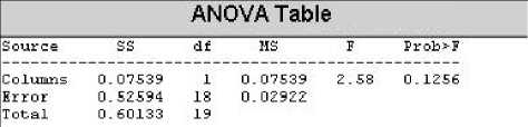
Figure 3: ANOVA table for radius 4 for IHR.

In the table above it is shown that f-value (2.58) is less than the f critical (4.41) indicating that there is no significant difference between the column three and the column four in the table and hence the optimum radius size can be used as 4 bpm. This radius size is used to calculate the CTM for all the records in this project.

The same procedure is followed to find out the optimum radius size for calculating CTM for BBI and for radius size .03 sec, the following result is obtained:

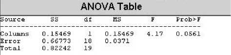
Figure 4: ANOVA Table for radius 0.03 for BBI.

results are compared.

• A.    Phase Space Portrait

Phase space portrait is a useful technique for nonlinear analysis of the ECG signals. Here in this project, phase space analysis has been used on BBI and IHR time series and the results are analyzed to see if any significant difference is found between normal and abnormal data series [8].

• B.    Phase Space Portrait for IHR

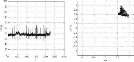
Following are the portraits obtained using phase space portrait on IHR. They are presented along with the IHR plot against each sample.

Here we can see that f-value (4.17) is less than the f critical (4.41) and hence the value of radius is set to 0.03 for measuring the CTM of BBI for all the records.

• D. Phase space portrait

Phase space or phase diagram is such a space in which every point describes two or more states of a system variable. The number of states that can be displayed in phase space is called dimension or reconstruction dimension. It is usually symbolized by the letter d or E. From the given digitized data x(1), x(2), …, x(n) of the IHR or BBI, a matrix A is obtained with its two columns given by x(1), x(2), …, x(n-τ) and x(1+ τ), x(2+ τ),.., x(n). Here τ is the time delay. The Phase space plot is constructed by plotting the data set with the time delay version of itself. The attribute of the reconstructed phase space plot depend on the choice of the value for τ. τ is measured through applying the autocorrelation function. Autocorrelation is a mathematical tool used frequently in signal processing for analyzing functions or series of values, such as time domain signals. Informally, it is a measure of how well a signal matches a time-shifted version of itself, as a function of the amount of time shift. More precisely, it is the cross-correlation of a signal with itself. Autocorrelation is useful for finding repeating patterns in a signal, such as determining the presence of a periodic signal which has been buried under noise, or identifying the missing fundamental frequency in a signal implied by its harmonic frequencies. τ is typically chosen as the time it takes the autocorrelation function of the data to decay to 1/e or the first minimum in the graph of the average mutual information. Here we used the two dimensional phase space portrait, i.e., d=2 [19, 20].

• V. Results and Discussion

Standard Deviation to assess the performance of the proposed method, we used the MIT-BIH Arrhythmia Database directory. The ECG signals in this directory were sampled at 360 Hz and with a quantization resolution of 11bits/sample. From this QRS complex locations, we determined BBI and hence IHR. From these BBI and IHR, the SD, CoV, CTM are determined for healthy persons as well as ailing persons and the

(a)                                    (b)

Figure 5: MIT-BIH Arrhythmia Record_100: (a) IHR(n) vs. Sample (n); (b) Phase space plot, with Lag, D=1. The patient has normal heart beat.

(a)                                    (b)

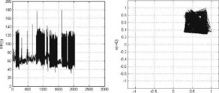
Figure 6: MIT-BIH Arrhythmia Record_106: (a) IHR(n) vs. Sample (n); (b) Phase space plot, with Lag, D=1. The patient has the following symptoms: Normal sinus rhythm, Ventricular bigeminy, Ventricular trigeminy.

C. Phase Space Portrait for BBI

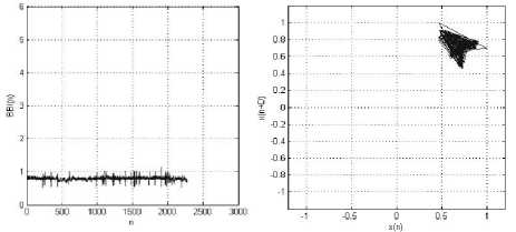
Following are the portraits obtained using phase space portrait on BBI. They are presented along with the BBI plot against each sample.

(a)

(b)

Figure 7: MIT-BIH Arrhythmia Record_100: (a) BBI (n) vs. Sample (n); (b) Phase space plot, with Lag, D=1. The patient has normal heart beat.

(a)                                    (b)

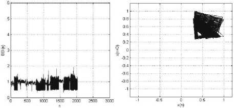
Figure 8: MIT-BIH Arrhythmia Record_106: (a) BBI (n) vs. Sample (n); (b) Phase space plot, with Lag, D=1. The patient has the following symptoms: Ventricular bigeminy, Ventricular trigeminy, and

Ventricular tachycardia.

The fact that the different parts of the single-cycle ECG wave mirror well understood physiological processes which are repeated with considerable precision introduces determinism-like properties in the ECG signal during the time between the beginning of the P-wave and the end of the T-wave. This motivates to the phase space portrait of the ECG signal in a two dimensional embedding space. The more closely spaced the data value are in the records, the more chance of having a fixed attractor with data lie on that. Since the normal rhythm shows more closely spaced R-R intervals, it is expected that most of the data will lie on a normal attractor and there will be a slight dispersion around that attractor. For abnormal rhythm records, the R-R intervals show more variation and hence their phase space portraits are expected to fill more of the 2-D plane and a random attractor should be obtained. From the phase space plot for both IHR and BBI, one can see that there lies significant difference between normal and abnormal rhythms. For the normal rhythm records like 100, 111, 112, 121, and 122, one can see that there is normal attractor which forms a slope of almost 45 degree with the axes and there is slight dispersion around that attractor. For the abnormal rhythm records like 106, 203, 221, 222, and 228, we can see that their phase space portrait fill more space in the plane and there is random attractor present in the plot [10].

• VI.    Statistical approach to data analysis

We determined the instantaneous heart rate (IHR) and the bit-to-bit interval (BBI) for eleven normal rhythm records as well as for eleven abnormal rhythms records. From these BBI and IHR data sets, the standard deviation (SD), coefficient of variation (CoV), central tendency measures (CTM) are determined and the results are shown in the table 1, 2, 3, and 4.

• A.    SD, CoV, and CTM for IHR

Table 1 shows the records of eleven healthy person’s ECG with the statistical analysis. The first column shows the record names. The second column provides the various bit types in those records in terms of number of minutes. The rest of the four columns show the Mean, SD, CoV, and CTM respectively determined from IHR of those records. Table 2 shows the same for eleven ECG records with abnormal rhythms.

T able .1 SD, C o V, CTM obtained from IHR of normal rhythm

Record	Mean	SD	CoV	CTM with r = 4 (bpm)
100	75.8104	5.0525	6.6647	0.6604
105	86.6585	10.9899	12.6818	0.6715
111	70.7966	3.9384	5.563	0.6671
112	84.45	2.5844	3.0603	0.8529
116	81.1354	10.4667	12.9003	0.7451
118	77.1806	10.9614	14.2022	0.7301
121	62.3587	6.2155	9.9674	0.9801
122	82.5183	4.5241	5.4826	0.8314
205	88.2911	8.2743	9.3716	0.8300
220	69.2941	12.0206	17.3472	0.8176
234	91.749	5.4253	5.9132	0.7345

T able .2 SD, C o V, CTM obtained from IHR of abnormal rhythm .

Record	Mean	SD	CoV	CTM with r = 4 (bpm)
106	75.228	27.2449	36.2164	0.2184
119	72.0917	22.5158	31.2322	0.2419
200	92.5029	22.7084	24.5488	0.0512
201	73.7016	29.2437	39.6785	0.0582
203	110.6457	37.2315	33.6493	0.0074
208	101.931	19.3936	19.0262	0.0518
210	88.3673	18.1342	20.5214	0.0438
219	75.6209	15.9812	21.1333	0.06
221	86.448	22.886	26.4737	0.0095
222	90.5739	29.0329	32.0543	0.0976
228	72.9255	19.2791	26.4367	0.1312

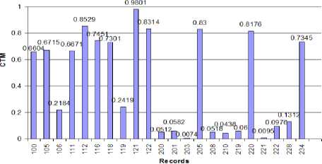
Figure 9: CTM for IHR plot against the record

Since the aim of applying CTM analysis is to differentiate between normal cardiac rhythm and cardiac abnormality, it is hoped that the CTM of abnormal IHR time series will be significantly different than that of normal one. First, looking at the standard deviations of the normal and abnormal IHR data series, one can see that there is a significant difference between them. For normal IHR data series, the standard deviation is low as expected whereas for abnormal IHR data series standard deviation is high. Same is true for coefficient of variation for both normal and abnormal IHR data series. When we analyze with the CTM, we find that CTMs of the normal IHR data series have high values with a mean of 0.7737 and SD 0.0946. On the other hand, CTMs of abnormal IHR data series have low values with the mean of 0.0883 and SD of 0.0748. Fig. 9 shows the plot of CTMs against their corresponding records. To observe the difference between the CTMs of normal and abnormal IHR data series, analysis of variance (ANOVA) technique is used. In the ANOVA technique, the f-value is calculated. It is seen that the CTM of the normal IHR data series is significantly different from that of the abnormal one, the f-value found to be 322.99 and the value of the f critical is 4.35 at 95% confidence level. This indicates that CTM can be used to differentiate between normal and abnormal IHR data series. Fig. 10 bellow shows the output of MATLAB anova1() function which represents the ANOVA obtained for the CTMs for normal and abnormal rhythms.

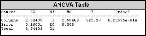
Figure 10: ANOVA table for CTM of IHR.

• B.    SD, CoV, and CTM for BBI

Table 5.3 shows the records of the same eleven healthy person’s ECG with the statistical analysis as described in the previous section. Table 5.4 shows the same for eleven ECG records with abnormal rhythms. These two tables show the analysis for BBI of the records.

T able .3 SD, C o V, CTM obtained from BBI of normal rhythm

Record	Mean	SD	CoV	CTM with r=0.03 (sec)
100	0.7946	0.0486	6.1163	0.4037
105	0.7012	0.0776	11.0651	0.6069
111	0.8499	0.0451	5.3113	0.331
112	0.7111	0.0218	3.0605	0.7918
116	0.7535	0.1904	25.2703	0.6297
118	0.7901	0.0975	12.3359	0.5785
121	0.9709	0.0912	9.39	0.6656
122	0.7293	0.0402	5.511	0.7141
205	0.6848	0.0625	9.1322	0.81
220	0.8815	0.0936	10.6164	0.4866
234	0.6557	0.0306	4.6737	0.7556

T able .4 SD, C o V, CTM obtained from BBI of abnormal rhythm

Record	Mean	SD	CoV	CTM with r = 0.03 (sec)
106	0.8904	0.2675	30.0399	0.0647
119	0.9084	0.2563	28.2114	0.1144
200	0.6898	0.1751	25.39	0.05
201	0.9503	0.3831	40.3136	0.0133
203	0.6058	0.2001	33.0367	0.0141
208	0.6142	0.1582	25.7504	0.0833
210	0.7086	0.1634	23.0656	0.0397
219	0.8379	0.2281	27.2171	0.0288
221	0.7444	0.2031	27.2883	0.0083
222	0.7278	0.2142	29.4369	0.0597
228	0.8734	0.2115	24.2197	0.0498

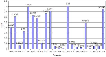
Figure 11: CTM for BBI plot against the records

Like the IHR of the records, BBI data series also shows the same behavior in terms of SD and CoV. Low SD and CoV are observed for normal BBI data series whereas high values of SD and CoV is seen for abnormal BBI data series. When analyzed with the CTM, normal BBI data series have high values with a mean of 0.6172 and SD 0.1472. On the contrary, CTMs of abnormal BBI data series have low values with the mean of 0.0478 and SD of 0.0308. Fig. 11 shows the CTM for BBI plot against the records. For the abnormal records 201, 203, 210, 219, and 221, where atrial fibrillation is prominent, we can find very low values of CTM ranging from 0.01 to 0.04. For abnormal records 106, 200, and 228, where ventricular bigeminy is the main abnormality, we find the CTM to be in the range of 0.05 to 0.065. For the records 119, and 208 where ventricular trigeminy is prominent, we find CTM with comparatively higher value of 0.083 to 0.12. To observe the difference between the CTMs of normal and abnormal BBI data series, analysis of variance (ANOVA) technique was used. It was seen that the CTM of the normal BBI data series is significantly different than that of the abnormal one, the f-value was found to be 143.31 and the value of the f critical is 4.35 at 95% confidence level. This indicates that CTM can differentiate between normal and abnormal BBI data series. Fig. 12 bellow is obtained using the MATLAB anova1() function for the CTMs from normal and abnormal rhythms.

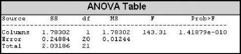
Figure 12: ANOVA table for CTM of IHR.

So, if we compare the two techniques we used namely phase space portrait and the central tendency measure, we can come out with the following facts. Phase space portrait only gives us a visual observation of the ECG signals, whether they are from normal or abnormal rhythms. On the contrary, central tendency measure quantifies the abnormality levels present in the ECG signals. Moreover, it roughly gives an idea about the abnormality type as observed in our work.

• VII.    Conclusion

In this work, effective ECG classification techniques are presented based on the underlying chaos in the system. The whole work is based on the fact that R-R intervals for normal rhythm data set tend to be invariant and that for the abnormal rhythm data set tend to vary a lot. This work describes the application of phase space portrait and CTM to differentiate the normal rhythm from the abnormal one. First IHR and BBI were calculated from the ECG of eleven normal rhythms as well as from that of eleven abnormal rhythms, each approximately 30 minutes in duration, and total twenty two data sets were constructed. Then CTM and phase space portrait were determined from those data sets and results are compared for normal and abnormal rhythm data sets. Phase space portrait of IHR and BBI for normal rhythm tends to demonstrate a normal attractor with a little deviation around it. Phase space portrait of IHR and BBI for abnormal rhythm demonstrate a widely dispersed plot which is a random attractor. Significantly low values of SD and CoV for normal rhythms are observed as compared to those for abnormal rhythms. The results show that there is a significant difference between the CTM of normal rhythm data sets and that of abnormal rhythm data sets. CTM for both IHR and BBI of normal rhythm data set tends to show very high value as compared to that of the abnormal rhythm data set as expected. Hence, we can easily classify normal and abnormal ECG records based on their underlying chaos. Moreover, for the BBI data set, we could roughly distinguish some types of abnormalities like atrial fibrillation, ventricular bigeminy, and ventricular trigeminy. However, we could not generalize this abnormality detection since we worked only with a limited number of records. Based on the computational simplicity and high levels of accuracy obtained by this technique, it is logical to use this approach to classify the ECG as normal or abnormal.

In this work, we have tried to classify ECG using the chaotic model of the system. We have shown that CTM and phase space portrait can distinguish between normal and abnormal cardiac rhythm. In this work, we determined the phase space portrait of the whole ECG record which contains both the normal and abnormal beats. Future work may include working with more number of abnormal records to generalize the detection of beat abnormality type.