Classification of Electroencephalographic Changes in Meditation and Rest: using Correlation Dimension and Wavelet Coefficients

Published Online April 2012 in MECS

Meditation is a practice of concentrated focus upon the breath in order to still the mind. Meditation in its various forms is a traditional exercise with a potential benefit on well-being and health. Many studies focused on the physiological effects of different meditation techniques to gain insight into the physiological prerequisites responsible for the improvement of health [1-4].

Analysis of Electroencephalogram (EEG) signals has provided a non invasive method for assessing brain activity. It was reported that during meditation, alpha and theta EEG power are increased, and autonomic response to external stimuli are reduced or enhanced [5-

• 9] . Furthermore, a number of literatures have reported the fruitful results of characterizing the dynamical behavior of the EEG signals during meditation [8-10].

• 2.    Background

  • 2.1    Data collection

Although EEG signals during meditation has been studied in the past [10-13], there remains a lack of significant effort on classifying these signals during rest and meditation.

Feature extraction is the determination of a feature or a feature vector from a pattern vector. The feature vector, which is comprised of the set of all features used to describe a pattern, is a reduced-dimensional representation of that pattern. The module of feature selection is an optional stage, whereby the feature vector is reduced in size including only, from the classification viewpoint, what may be considered as the most relevant features required for discrimination. In the feature extraction stage, numerous different methods can be used so that several diverse features can be extracted from the same raw data. In this study, Wavelet coefficients and Correlation dimension are considered as the feature vectors.

The outline of this study is as follows. In the next section, we briefly describe the set of EEG signals used in our study. Then, an algorithm was presented to classifying rest and meditation by using EEG signals. In this algorithm, after preprocessing of EEG signal in three channels (Fz, Cz and Pz), Wavelet coefficients and Correlation dimension are extracted. After that, some parametric and nonparametric classifiers are used to classify the EEG signals. Finally, the results of present study are shown and the study is concluded.

Twenty five subjects took part in the study. Fifteen subjects: eleven meditators (mean age 40.18±7.19, mean meditation experience 5 to 7 years) and four non- meditators (mean age 25.5±1.91) were asked to do meditation by listening to the guidance of the master.

The other ten subjects were asked to do meditation by themselves. They were considered to be at an advanced level of meditation training (mean meditation experience 7 years, mean age 37.8±6.39). The subjects were in good general health and did not follow any specific heart diseases. The subjects were asked not to eat salty or fat foods before meditation practices or data recording. Informed written consent was obtained from each subject after the experimental procedures had been explained [8-9].

The experimental procedure was divided into two different stages: Subjects were first instructed to sit quietly for 5 minutes and kept their eyes closed. After that, they performed meditation. Meditation prescribes a certain bodily posture. They sit on a cushion 5 to 10 centimeters thick that is placed on blanket. They cross their legs so that one foot rests on the opposite thigh with the sole of their foot turned up and with their knees touching the blanket (lotus or half-lotus position). The torso should be kept straight, but it should not be strained. The head should be kept high with eyes closed. During this session, the meditators sat quietly, listening to the guidance of the physician and focusing on the breath [8-9].

The meditation EEG signals were recorded in meditation clinic using 16-channel Powerlab (manufactured by ADInstruments). EEG activity was recorded using three electrodes (i.e., Fz, Cz and Pz) according to the International 10–20 System, referenced to linked ear lobe electrodes (Fig. 1). The monitoring system hardware filters band passed data in range: 0.150 Hz for EEG time series. A digital notch filter was applied to the data at 50Hz to remove any artifacts caused by alternating current line noise. The sampling rate was 400Hz.

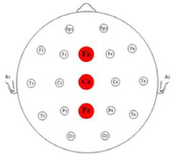
Figure 1. EEG electrodes possitions

• 2.2    Feature extraction

  • 2.2.1    Wavelet transform

The multi-scale feature of the Wavelet transform (WT) allows the decomposition of a signal into a number of scales, each scale representing a particular coarseness of the signal under study. The procedure of multi-resolution decomposition of a signal x[n] is schematically shown in Fig. 2.

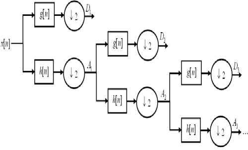
Figure 2. Sub-band decomposition of discrete Wavelet transforms implementation; g[n] is the high-pass filter, h[n] is the low-pass filter

Each stage of this scheme consists of two digital filters and two down-samplers by 2. The first filter, g[.] is the discrete mother Wavelet, high-pass in nature, and the second, h[.] is its mirror version, low-pass in nature. The down-sampled outputs of first high-pass and low-pass filters provide the detail, D 1 , and the approximation, A 1 , respectively. The first approximation, A 1 , is further decomposed and this process is continued as shown in Fig. 2.

All WTs can be specified in terms of a low-pass filter, h, which satisfies the standard quadrature mirror filter condition:

H ( z ) H ( z - 1 ) + H ( - z ) H ( - z ^{- 1} ) = 1 ⁽¹⁾

where H(z) denotes the z-transform of the filter h. Its complementary high-pass filter can be defined as:

G (z) = zH (- z-1)

A sequence of filters with increasing length (indexed by i) can be obtained

Hi+i (z) = H^z2i Hi (z)

G i + i ( z ) = G ^ z ² i j H i ( z ), i = 0, к , I - 1

with the initial condition H0(z) = 1. It is expressed as a two scale relation in time domain hi+1(k) = [h]T2i * hi(k)

^G i + 1 ⁽ k ) = ^[ g ] T 2 i * h i ⁽ k )

where the subscript [,] t m indicates the up-sampling by a factor of m and k is the equally sampled discrete time. The normalized Wavelet and scale basis functions φ i,l (k) and ψ i,l (k) can be defined as:

^ i,l ( k ) = 2 ^i/2 h i ( k - 2 i l ) ⁽⁵⁾ _V i,l ( k ) = 2 i/2 g i ( k - 2 i l )

where the factor 2i/2 is an inner product normalization, i and l are the scale parameter, and the translation parameter, respectively. The discrete Wavelet transform (DWT) decomposition can be described as:

a (i) ^{( l} ) = x ⁽ k ) * Р Ц ⁽ k ) ⁽⁶⁾ d (i) ⁽ l ) = x ⁽ k ) * V i,l ⁽ k )

where a (i) (l) and d (i) (l) are the approximation coefficients and the detail coefficients at resolution i, respectively [14].

The biological signals can be considered as a superposition of different structures occurring on different time scales at different times [15]. One purpose of Wavelet analysis is to separate and sort these underlying structures of different time scales. Selection of appropriate Wavelet and the number of decomposition levels are very important in analysis of signals using the WT. The number of decomposition levels is chosen based on the dominant frequency components of the signal. The levels are chosen such that those parts of the signal that correlate well with the frequencies required for classification of the signal are retained in the Wavelet coefficients. Usually, tests are performed with different types of Wavelets and the one which gives maximum efficiency is selected for the particular application. In the present study, the number of decomposition levels was chosen to be four. Thus, the EEG signals were decomposed into the details D₁ - D₄ and one final approximation, A 4 .

The dimension D 1 is called the dimension. This is defined by (9),

M(r)

7 . , P i logp i

D1 = limD2 = lim——-------, q^1     r^0     log Г

The dimension D2 is called the

Dimension. This can be written as (10):

logC(r)

D 2 = lim—-—— r ^ o logr

M(r)

C(r) = 7 p 2

1 = 1

2.2.2 Correlation dimension

A fractal dimension D is any dimension measurement that allows non integer values [16]. A fractal is a set with a non integer fractal dimension. Standard objects in Euclidean geometry are not fractals but have integer fractal dimensions D=d. The primary importance of fractals in dynamics is that strange attractors are fractals and their fractal dimension D is

simply related to the minimum number of dynamical variables needed to model the dynamics of the strange attractor.

The simplest way (conceptually) to measure the

dimension of a set is to measure the Kolmogorov capacity (or box-counting dimension). In this

measurement a set is covered with small cells (e.g.,

squares for sets embedded in two dimensions, cubes for

sets embedded in three dimensions) of size ε. Let M(ε)

denote the number of such cells that contain part of the

set. The dimension is then defined as (7):

D = lim

£^^

log(M( e )) ^log ⁽ V ^e)

More elaborate dimension measurements are available that take into account in homogeneities or Correlations in the set. The dimension spectrum defined by Hentschel and Procaccia [16],

M(r) log p^q

Dq = lim—--^^кЛ, q t^o q -1     log r

q = 0,1,2, к

information

Correlation

C(r) is the Correlation sum, which is essentially (exact in the limit N→∞) the probability that two points of the set are in the same cell.

For a given set, the dimensions are ordered D 0 ≥ D 1

≥ D 2 ≥ …. If the set is a homogeneous attractor then

^pi = M

The major difficulty in calculating D q is the practical difficulty of covering the set with cells of very small size. In general, this requires too much computer storage and time to obtain convergence to a limit r→0.

When q=2 the dimension estimate can be made computationally tractable by using an algorithm proposed by Grassberger and Procaccia [16].

Grassberger-Procaccia algorithm

The Grassberger-Procaccia algorithm [16] is based on the following approximation: The probability that two points of the set are in the same cell of size r is approximately equal to the probability that two points of the set are separated by a distance ρ less than or equal to r. Thus C(r) is approximately given by (13):

_n E Nj > i ® ( ^{r -p( x} i ,x j ))

C(r)»—i---------

₂n(n - 1 )

Where the Heaviside function is defined as (14):

f l     if s >  0                                 (14)

® ( s ) =)

[ 0     if s <  0

The approximation in (13) is exact in the limit N→∞; however, this limit cannot be realized in practical applications. The limit r→0 used in the definition of D 2 is also not possible in practice. Instead, Procaccia and Grassberger propose the (approximate) evaluation of C(r) over a range of values of r and then deduce D 2 from the slope of the straight line of best fit in the linear scaling region of a plot of log C(r) versus log r.

The most common metric employed to measure the distance ρ in (13) is the Euclidean metric,

m

E(xi(k)- xj(k ))2

V k =1

The choice of metric should not affect the scaling of the Correlation sum with r.

provides a set of fractal dimension measurements that take into account higher order Correlations as q is increased.

• 2.3    Classification

• 2.3.1    Fisher's discriminant

In this paper, the Correlation dimension and Wavelet coefficients are used as inputs of four different classifiers. The task at hand is to classify the EEG epochs of twenty five healthy women as either related to before or to during meditation. The four different classification methods are Fisher classifier, Quadratic classifier, k-Nearest Neighbour (k-NN) and Parzen classifiers.

Statistical classifiers fall into two categories; parametric and non-parametric [17]. The linear and Quadratic classifiers are of the parametric type. In this type, the classification rules are based on models of the probability density function of the data. Both Linear and Quadratic classifiers are based on the assumption that classes have multivariate Gaussian distributions.

The k-NN is a nonparametric classification procedure and hence no assumption of the form of the underlying densities is required. This method, however, assumes that there are enough points from each class such that in any small region within the decision space, the number of points occurring in these regions indicates the true nature of each density function.

The description of each classifier models that are considered in this study are presented in the following sections.

The terms Fisher's linear discriminant and linear discriminant analysis (LDA) are often used interchangeably, although Fisher's original article [18] actually describes a slightly different discriminant, which does not make some of the assumptions of LDA such as normally distributed classes or equal class covariances.

Suppose two classes of observations have means Xy = 0, /y = 1, and covariances Ey = 0, Ey = 1. Then the linear combination of features or. r will have means or. / v=i and variances orT 7 or for i = 0,1. Fisher y                    y—iy=i defined the separation between these two distributions to be the ratio of the variance between the classes to the variance within the classes:

S = ^between = Jo^^-°!lXiy=0)L с2 ,.    or T У or + or T У or within       y_jy=1      y_jy=0

Й- ^X y = 1 - X y = 0 )P

" or T fy   +У L

(■^ y = 1    y - 0y = 0 )

This measure is, in some sense, a measure of the signal-to-noise ratio for the class labeling. It can be shown that the maximum separation occurs when f             y1

^o = IX 1 + У A I I ^х y = 1 - ^Xy = 0 '

( ^^y = 1    ^^y = 0 )

When the assumptions of LDA are satisfied, the above equation is equivalent to LDA.

Be sure to note that the vector or is the normal to the discriminant hyperplane. As an example, in a two dimensional problem, the line that best divides the two groups is perpendicular to or.

Generally, the data points to be discriminated are projected onto o r ; then the threshold that best separates the data is chosen from analysis of the one-dimensional distribution. There is no general rule for the threshold. However, if projections of points from both classes exhibit approximately the same distributions, a good choice would be the hyperplane between projections of the two means, o r . / y = 0 and o r . / y = 1 . In this case the parameter c in threshold condition o r . x <  c can be found explicitly:

c = < ° . ^{( x} y = 0 ⁺ Zr y = 1)/ ² (18)

• 2.3.2    Quadratic classifier

A Quadratic classifier is used in machine learning and statistical classification to separate measurements of two or more classes of objects or events by a Quadratic surface. It is a more general version of the linear classifier.

Quadratic discriminant analysis (QDA) is closely related to LDA, where it is assumed that the measurements from each class are normally distributed. Unlike LDA however, in QDA there is no assumption that the covariance of each of the classes is identical. When the normality assumption is true, the best possible test for the hypothesis that a given measurement is from a given class is the likelihood ratio test.

Suppose there are only two groups, (so y e {0,1}), and the means of each class are defined to be μ y = 0, μ y = 1 and the covariances are defined as Σy = 0, Σy = 1. Then the likelihood ratio will be given by

Likelihood ratio = (19)

I -------------------1

2 п У j        y = 1

- 1

2 п У ^—1 y = 0

f expl- ^ (x - Xy =1

'T g=, ( x - x y = 1 ) )

) T Z -t » ( x - X y *) )

< t

f expl - ^ (x - Xy=0

for some threshold t. After some rearrangement, it can be shown that the resulting separating surface between the classes is a Quadratic. The sample estimates of the mean vector and variance-covariance matrices will substitute the population quantities in this formula.

• 2.3.3    K-nearest neighbour classifier

• 2.3.4    Parzen classifier

• 3.    Results

In pattern recognition, the k-nearest neighbor algorithm (k-NN) is a method for classifying objects based on closest training examples in the feature space. K-NN is a type of instance-based learning, or lazy learning where the function is only approximated locally and all computation is deferred until classification. The k-nearest neighbor algorithm is amongst the simplest of all machine learning algorithms: an object is classified by a majority vote of its neighbors, with the object being assigned to the class most common amongst its k nearest neighbors (k is a positive integer, typically small). If k = 1, then the object is simply assigned to the class of its nearest neighbor.

The same method can be used for regression, by simply assigning the property value for the object to be the average of the values of its k nearest neighbors. It can be useful to weight the contributions of the neighbors, so that the nearer neighbors contribute more to the average than the more distant ones (A common weighting scheme is to give each neighbor a weight of 1/d, where d is the distance to the neighbor. This scheme is a generalization of linear interpolation).

The neighbors are taken from a set of objects for which the correct classification (or, in the case of regression, the value of the property) is known. This can be thought of as the training set for the algorithm, though no explicit training step is required. The k-nearest neighbor algorithm is sensitive to the local structure of the data.

Nearest neighbor rules in effect compute the decision boundary in an implicit manner. It is also possible to compute the decision boundary itself explicitly, and to do so in an efficient manner so that the computational complexity is a function of the boundary complexity [19].

The Parzen classifier provides an estimate of the class-conditional probability density function (PDF) by, e.g., applying a kernel density estimator to the labeled feature vectors in the training set, while a Gaussian Mixture Model (GMM) classifier estimates classconditional PDFs using mixtures of multivariate normal PDFs [20].

The Parzen classifier estimates the class densities by the Parzen density estimation and has a built-in optimization for the smoothing parameter.

Features play an important role in classifying systems. Features are selected based on either best representation of a given class of signals or best distinction between classes. High-dimension of feature vectors increased computational complexity and the classifier trained on these feature vectors produced lower accuracy.

In this study, Correlation dimension and Wavelet coefficients of EEG signals in Fz, Cz and Pz were estimated. Then the results of analysis of EEG signals during meditation were compared to before meditation.

Two features in Wavelet domain are extracted: the approximate and detail Wavelet coefficients at the forth decomposition level of EEG signals (Fz, Cz and Pz channels). Therefore, these six composite features are used as an input of four different classifiers.

In the next stage, Correlation dimensions, as nonlinear features, are extracted from the three channels of EEG signals and then input into the classifiers.

Fisher's discriminant, k-NN classifier, Quadratic classifier and Parzen classifier proposed for classification of EEG features were implemented by using MATLAB software package (MATLAB with PRTOOLS toolbox).

The epochs in the data set were randomly divided into two sets: a training set and a testing set. 70% of the epochs are used to train the classifiers while 30% were used to test the performance of each classifier.

The values of classification accuracy, classification error and the central processing unit (CPU) times of training of the four classifiers trained on Wavelet coefficients and Correlation dimensions are presented in Table I and Table II, respectively.

TABLE I. Classification results on wavelet coefficients.

Classifier	Accuracy (%)	Error	Elapsed time(s)
Fisher	85.02	0.25	5
Quadratic	82.55	0.3	3
k-NN	81.06	0.32	60
Parzen	84.75	0.25	35

TABLE II. Classification results on correlation dimensions.

Classifier	Accuracy (%)	Error	Elapsed time(s)
Fisher	92.37	0.25	4
Quadratic	90.27	0.29	5
k-NN	89.29	0.36	54
Parzen	92.37	0.25	34

The classification results presented in Table I and Table II denote that the Fisher discriminant and Parzen classifier trained on both composite features obtain higher accuracy than that of the others. The total classification accuracy of the Fisher discriminant and Parzen classifier applying Wavelet coefficients was 85.02% and 84.75%, respectively which is raised to 92.37% in both classifiers using Correlation dimensions. As it can be observed, the parametric classifiers give good results.

As mentioned above, these classifiers are based on the assumption that classes have multivariate Gaussian distributions. Probability density function (PDF) of Correlation dimension of EEG signals in Fz channel during meditation is shown in Fig. 3.

PDF of Correlation Dimension

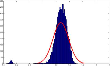
Figure 3. Probability density function (PDF) of Correlation dimension in Fz channel during meditation

• 4.    Conclusion

In this study, in order to classify rest and meditation signals, a new application of parametric and nonparametric classifiers employing different features is presented. For the first time in this investigational field, we had done a feature extraction using Correlation dimension and Wavelet coefficients in certain psychological state (meditation and rest) assessment.

Two features in Wavelet domain (the approximate and detail Wavelet coefficients at the forth decomposition level) and Correlation dimensions of EEG signals in Fz, Cz and Pz channels are extracted.

Four different classifiers were used to classify two classes of EEG signals (before and during meditation) when the Wavelet coefficients were used as inputs. The same process was done for Correlation dimensions.

The results demonstrate that the Fisher discriminant and Parzen classifier trained on both composite features obtain higher accuracy than that of the others. Although, the accuracy of the classifiers are improved by using nonlinear features (Table II). The total classification accuracy of the Fisher discriminant and Parzen classifier applying Correlation dimensions reach to 92.37% in both classifiers.

We therefore have concluded that the proposed classifiers trained on Correlation dimension can be used in detecting electroencephalographic changes in specific psychological states.

Some future work should also be carried out. For instance, other classification techniques, such as neural networks, can be used to obtain efficient and accurate results in the future.

Acknowledgements

We thank Dr. Minoo Morvarid, the Master of Meditation Clinic in Mashhad, and Ms. Shahla Khoshkholgh for their assistance in collecting the data that were used in the investigations. The authors would also like to thank all the subjects for their good collaborations.