Clustering Structure and Deployment of Node in Wireless Sensor Network

Published Online September 2014 in MECS DOI: 10.5815/ijitcs.2014.10.10

• I.    Introduction

  In current years, the WSN has important applications such as remote environmental monitoring and target tracking. After the publication of Ian F. Akyildiz, Weilian Su, Yogesh Sankarasubramaniam, and Erdal Cayirci, and survey on sensor networks, IEEE Communications Magazine, 2002. We give an overview of several new applications and then various aspects of WSNs. We classify the problems into three different categories:

• >    The internal platform and principal operating system, >  The communication protocol stack,

• >    The network services, provisioning, and deployment.

The Micro Electro Mechanical Systems (MEMs) technology developed the smart sensors. The smart sensors are small, with limited processing and computing resources, and they are low-cost compared to traditional sensors. These smart sensor or sensor nodes can sense, measure, and gather information from the environment and, based on some local decision process, they can transmit the sensed data to the user. Example of some sensors can sense light, can sense pressure some can sense temperature simultaneously.

The WSN nodes have to be improved by integrating actuators. Actuators can be simple devices programmed to take immediate, one-shot, action in response to sensory input, or they can be more sophisticated entities (like robots) that interact with their environment in more complex ways.

The smart SNs are low power devices equipped with one or more sensors, a processor, memory, a power supply, a radio, and an actuator. A variety of mechanical, thermal, biological, chemical, optical, and magnetic sensors may be attached to the sensor node to measure properties of the environment. Since the sensor nodes have limited memory and are typically deployed in difficult-to-access locations, a radio is implemented for wireless communication to transfer the data to a BS (e.g., a laptop, a personal handheld device, or an access point to a fixed infrastructure). Battery is the main power source in a sensor node. Secondary power supply that harvests power from the environment such as solar panels may be added to the node depending on the appropriateness of the environment where the sensor will be deployed. Depending on the application and the type of sensors used, actuators may be incorporated in the sensors. Typically, a WSN has little or no infrastructure. It consists of a number of sensor nodes (few tens to thousands) working together to monitor a region to obtain data about the environment. There are two types of WSNs:

• a.    Structured WSN and

• b.    Unstructured WSN.

• A.    Structured WSN

In a structured WSN, all or some of the SNs are deployed in a fixed location. The advantage of a structured network is that fewer SNs can be deployed with lower network maintenance and management cost. Fewer nodes can be deployed now since SNs are placed at specific locations to provide coverage while ad-hoc deployment can have uncovered regions.

• B.    Unstructured WSN

An unstructured WSN is one that contains a dense collection of SNs. The SNs may be deployed in an ad-hoc manner into the field. Once deployed, the network is left unattended to perform monitoring and reporting functions. In an unstructured WSN, network maintenance such as managing connectivity and detecting failures is difficult since there are so many SNs. In generally, a WSN consists of a host or “gateway” that communicates with a number of wireless sensors (or SNs) via a radio link. Data is collected at the SNs, compressed, and transmitted to the gateway directly. If the data is required then uses the SNs. Otherwise, SNs to forward data to the gateway. The gateway then ensures that the data is input into the system. Each wireless sensor is considered a node which presents wireless communication capability, along with a certain intelligence for signal processing and networking data. Depending on the type of application, each node can have a specific address. That is shown in fig.1.

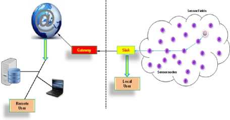
Fig. 1. The Sensor in WSN.

• 1.    Types of sensor networks

Generally, the WSNs are deployed on land, underground, and underwater. There are five types of WSNs:

• a.    terrestrial WSN,

• b.    underground WSN,

• c.    underwater WSN,

• d.    multi-media WSN, and

• e.    mobile WSN.

• a.    terrestrial WSN

A network consists of hundreds to thousands of sensor nodes deployed on land. The challenges are in network data aggregation to improve performance across communication, delay, minimizing energy cost, reduce the amount of data communication, finding the optimal route, distributing energy consumption, maintaining network connectivity and eliminating redundancy. The terrestrial WSN applications are environmental sensing and monitoring, industrial monitoring, surface explorations.

• b.    underground WSN

A network consists of wireless SNs deployed in caves or mines or underground. The challenges are expensive deployment maintenance and equipment cost, threats to device such as the environment and animals, battery power cannot easily be replaced, topology challenges with pre-planned deployment, high levels of attenuation and signal loss in communication. The underground WSN applications are agriculture monitoring, landscape management, underground structural monitoring, military border monitoring and underground environment monitoring of soil, water or mineral.

• c.    underwater WSN

A network consists of wireless sensor and vehicles deployed into the ocean environment. The challenges are expensive underwater sensors, hardware failure due to environment effects (e.g., corrosion), battery power cannot easily be replaced, sparse deployment, limited bandwidth, long propagation, delay, high latency, and fading problems. The underwater WSN applications are pollution monitoring, undersea surveillance, and exploration, disaster prevention monitoring, seismic monitoring, equipment monitoring, and underwater robotics.

• d.    multi-media WSN

A network consists of wireless sensor devices that have the ability to store, process, and retrieve multi-media data such as video, audio, and images. The challenges are innetwork processing, filtering, and compressing of multimedia content, high energy consumption and bandwidth demand, deployment based on multi-media equipment coverage, flexible architecture to support different applications, must integrate various wireless technologies, QoS provisioning is very difficult due to link capacity and delays and effective cross-layer design. The multimedia WSN applications are enhancement to existing applications such as tracking and monitoring.

• e.    mobile WSN

• 2.    WSN applications

A network consists of mobile SNs that have the ability to move. The challenges are navigating and controlling mobile nodes, must self-organized, localization with mobility, minimize energy cost, maintaining network, connectivity, in network data processing, data distribution, mobility management, minimize energy usage in locomotion, maintain adequate sensing coverage. The mobile WSN applications are environmental monitoring, habitat monitoring, military surveillance, target tracking, underwater monitoring, search and rescue in [1].

In [2], it can be classified into two categories one is monitoring and another is tracking. The monitoring applications include indoor/outdoor environmental monitoring, health and wellness monitoring, power monitoring, inventory location monitoring, factory and process automation, and seismic and structural monitoring. Tracking applications include tracking objects, animals, humans, and vehicles. While there are many different applications, below we describe a few example applications that have been deployed and tested in the real environment shown in fig.2.

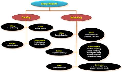
Fig. 2. The overall view of WSN applications

The rest of this paper is structured as follows. The review of the literature is followed in Section 2, The proposed methodology is formulated in Section 3. Section 4 discusses the sensor node clustering structures. Section 5 discusses the experimental and analysis results of the proposed methodology. Finally, conclusions are given in Section 6.

• II.    Sensor Node

A sensor node was developed in North America. A sensor node also known as a “mote”. It is a node in a wireless sensor network that is capable of performing some processing, gathering sensory information and communicating with other connected nodes in the network. A mote is a node but a node is not always a mote. There are two types of SNs used in the WSN. One is the normal sensor node deployed to sense the phenomena and the other is gateway node that interfaces sensor network to the external world. The main architecture of sensor node includes following components:

• >    Controller module

• >    Memory module

• >    Communication module

• >    Sensing modules

• >    Power supply module.

The one or more SNs gather data from the environment. The central unit, a microprocessor, manages the tasks. A transceiver communicates with the environment and a memory is used to store temporary data or data generated during processing. Data processing tasks are often spread over the network, i.e. nodes co-operate in transmitting data to the sinks (Verdone et al., 2008). The battery supplies all parts with energy, and energy efficiency is crucial. Although most sensor nodes have a traditional battery, there is some early stage research on the production of sensors without batteries, using technologies similar to passive RFID chips shown in fig. 3.

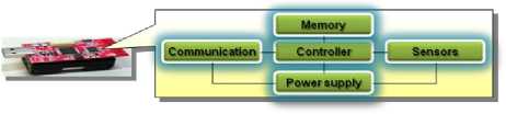
Fig. 3. The components of sensor nodes

• III.    Wsn Architectures

As per the data are collected, WSNs can be classified into three types:

• A.    Homogenous sensor networks,

• B.    Heterogeneous sensor networks, and

• C.    Hybrid sensor networks

• A.    Homogenous sensor networks

A homogenous network consists of base stations and sensor nodes  equipped with equal  capabilities  of computational power  and  storage capacity.   In homogenous network, there are two topologies structures.

• a.    Flat Topology Network and

• b.    Hierarchical Topology Network.

• a.    The flat topology network

In this network, data aggregation is accomplished by data centric routing where the BS usually transmits a query message to the SNs via flooding, and the SNs that have data matching the query will send response messages back to the base station. The SNs communicate with the BS via multi-hop routes by using peer nodes as relays. The choice of a particular communication protocol depends on the specific application [2]. The fig. 4 showed the architecture of a flat network. The SNs are assumed to be stationary once being distributed in the targeted area and the collected sensing information is gathered at the BS.

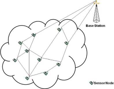
Fig. 4. The flat Topology Network

• b.    The hierarchical topology network

In a hierarchical topology network, SNs are organized into clusters where the CHs serve as simple relays for transmitting the data. Since the CHs have the same transmission capacity as the SNs, the minimum requirement on the number of clusters can be derived from the upper bound of the throughput. Higher throughput can be achieved by using clustering at the cost of having extra nodes functioned as CHs. Data aggregation in a hierarchical network involves data fusion at CHs, which reduces the number of messages transmitted to the BS, and hence improves the energy efficiency of the network. A typical structure of a hierarchical network is shown in fig.5.

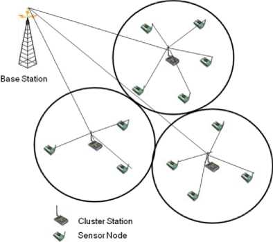
Fig. 5. The hierarchical topology

• B.    Heterogeneous sensor networks

A heterogeneous sensor network consists of two important components one is BSs (fixed and mobile) and sophisticated SNs with advanced embedded processing and communicating capabilities. In [3], the data gathering can be executed at the mobile BSs. The mobile base stations move randomly in the area of the deployed network, collecting data directly from normal sensor nodes, or use some surrounding SNs to relay the data as shown fig.6. Again in [4], sometimes, SNs may be distributed sparsely and the distance between any two SNs can be far apart. The long distance among SNs implies that more energy will be consumed for communication. Meanwhile, SNs need to perform sensing and communication for as long as possible. The data gathering with mobile sinks is able to prolong the lifetime of the system.

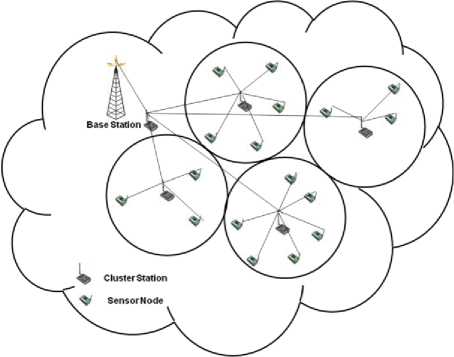
Fig. 6. Heterogeneous sensor network topology

• C.    Hybrid sensor networks

In this network, the several mobile BSs work cooperatively to provide fast data gathering in a real time manner. In the development shown in fig.7, collected data will be relayed by several mobile base stations. The conventional and well studied routing algorithms for ad hoc networks can be adopted as the routing protocols among these mobile BSs. The MANETs assume that every node is able to move at their own pace. Even though WSNs are more constrained than other wireless networks, for example, MANETs, in terms of energy, processing, transmission range, and bandwidth, routing from a source BS to a destination BS can be accomplished by using MANET protocols in hybrid sensor networks [2]. Accordingly, if the location of a BS is unpredictable or in case the BSs cannot communicate with each other on their own, it is reasonable to tailor techniques originally proposed for MANETs and apply them in WSNs. Hybrid sensor networks can achieve longer lifetime and can also improve the efficiency of data gathering [3,5]. As pointed out in [6], a mobile BS prefers the hybrid architecture, by which a mobile BS can communicate with other sensor nodes by using a WSN protocol and with other BSs by using a MANET protocol. While individual sensor nodes are not as powerful as normal computers, a large number of sensor nodes are required to provide high quality and reliable networking service, as well as easy deployment and fault tolerance in inaccessible environments where maintenance is inconvenient or impossible. Such unique operating environments and performance requirements of WSNs require fundamentally new approaches to networking design.

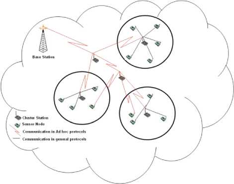
Fig. 7. The Hybrid sensor network topology

• IV. The Sensor Node Clustering Structures

In the WSN, the clustering mechanisms have been applied to sensor networks with hierarchical structures to enhance the network performance while reducing the necessary energy consumption [7]. Clustering is a crosscutting technique that can be used in nearly all layers of the protocol stack. The primary idea is to group nodes around a CH that is responsible for state maintenance and inter-cluster connectivity.

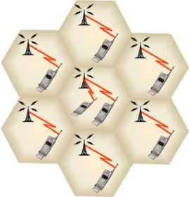
Fig. 8. Cluster structure in cellular system

In cellular networks, fixed BSs are connected through wired backbones. Communications between two mobile SNs that are only 1-hop away from their respective BSs can be established through the fixed base stations and the wired backbone. In this case, clustering is used to select and allocate channel groups to all the BSs within a system and to achieve efficient frequency reuse as shown in fig. 8. In multi-hop wireless networks, SN clustering is a technique that aggregates nodes into groups (clusters) to reduce the routing overhead and to provide a convenient framework for efficient resource (e.g., bandwidth or code) allocation, energy management, fault-tolerant routing, and high end-to-end throughput.

In clusters without any CH, a proactive strategy is used for intra-cluster routing while a reactive strategy is used for inter-cluster routing. However, as the network size grows, there will be heavy traffic overhead within the network [8]. Therefore, normally one node is selected as the cluster head of a cluster, and it acts as the local coordinator of transmissions within its cluster. A hierarchical routing or network management protocol can be more efficiently implemented with CHs. As compared to the base stations used in current cellular systems, the cluster head does not have any special hardware, and is in fact dynamically selected among the set of nodes. However, a cluster head performs additional functions as a central administration point, and a CH failure would degrade the performance of the entire network; it may become the bottleneck of the cluster. An efficient nodeclustering mechanism tends to preserve its structure when a few nodes are moving and the topology is slowly morphing. The objective of the node clustering procedure is to find a feasible interconnected set of clusters that covers the entire node population.

• A. Deployment of node in wsn

In WSN, the SNs could be deployed in the coverage area regularly or randomly.

• a.    Regularly placed nodes deployment

If the area to be deployed is easily accessible and sensor nodes can be placed anywhere, regular placement will allow the best possible coverage and easier clustering of the sensor nodes shown in fig. 9 and 10.

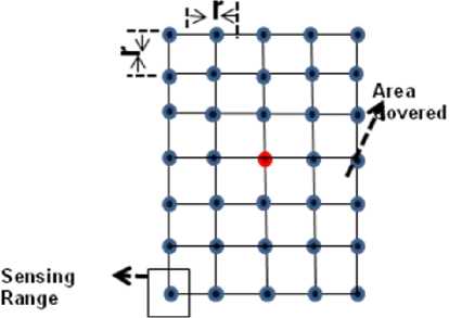
Fig. 10. Rectangular Deployment

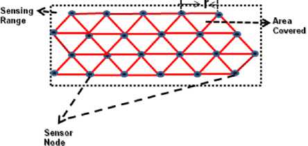
Fig. 9. Triangular Deployment

Table 1. Coverage area by each node and total required number of nodes for a given area A with adjacent distance between nodes R.

Cluster Shape	Distance between Adjacent Nodes	Coverage area by Each Node	Total Required number of Nodes per overage Area
Triangle	R	3 R2 4			4 A 3 R 2
Rectangular	R	R2			" A " R 2
Hexagonal	R	3 3 R2 4			4 A 3 3 R 2
Pentagonal	R	R 2 725 + 107s		4 A
		4		r 2/25 + 10V5
Octagonal	R	2(1 + 22 ) R 2		---4A--- 2(1 + 22) R2

To cover a given area A , assuming that the distance between any adjacent SNs is given by R in all cases, the coverage area of each SN and the total numbers of SNs required for three common placement types, triangular, rectangular, hexagonal, pentagonal, and octagonal clusters are given in Table 1. If each sub-region can be covered by more than one SN, some selected SNs can be allowed to go into the sleep state.

• b.    Randomly distributed nodes deployment Definition Poisson distribution

The Poisson distribution is a discrete probability distribution that expresses the probability of a number of events occurring in a fixed period of time if these events occur with a known average rate and independently of the time since the last event. The Poisson distribution can also be used for the number of events in other specified intervals such as distance, area or volume.

In the 1781–1840, the distribution was discovered by Siméon-Denis Poisson and published, together with his probability theory, in 1838 in his work Recherches surla probabilité desjugements en matières criminelles et matière civile ("Research on the Probability of Judgments in Criminal and Civil Matters"). The work focused on certain random variables N that count, among other things, a number of discrete occurrences (sometimes called "arrivals") that take place during a time-interval of given length. If the expected number of occurrences in this interval is λ, then the probability that there are exactly k occurrences (k being a non-negative integer, k = 0, 1, 2 ...) is equal to f (k; 2) = Pr (X = k) =

k - 2

2 e

k !

Where,

• •    e is the base of the natural logarithm ( e =2.71828...).

• •    k is the number of occurrences of an event-the probability of which is given by the function.

• •    k ! is the factorial of k.

• •    Z is a positive real number, equal to the expected number of occurrences that occur during the given interval.

As a function of k , this is the probability mass function. The Poisson distribution can be derived as a limiting case of the binomial distribution. The Poisson distribution can be applied to systems with a large number of possible events, each of which is rare. Many other applications of Poisson noise have been developed, e.g., estimating the node density of uniformly distributed over an area.

P r (N t = k ) = f ( k ; A t ) = e " ( " ) k           (2)

k !

In WSN, the nodes to be deployed are randomly distributed in an unknown or inaccessible area with unmanned devices or airplanes. In this state, the SNs have to discover their neighbors by themselves. If N nodes are uniformly distributed over an area A, the node density can be given by λ = N/A [9]. The probability that there are m SNs within the area S is Poisson distributed and can be given by

(AS) m

P (m ) = -—— e(3)

m !

The probability that the monitored area has one SN can be expressed as

P,-node = 1 - P(0) = 1 - e-"S(4)

In many situations, it needs at least k SNs cooperating within an area to ensure reliable service. The probability of having k nodes in a given area S can be expressed by k-1

P. - .odes = 1 -I P (m) = Z m=0

( A S ) m „- A S

m !

The sensing and communication ranges in a randomly distributed SNs deployment are determined by the maximum distance between any two adjacent SNs in the given area. Several heuristic deployment schemes have been discussed in [10].

V. The Experiment and Analysis

• A.    Results of Regularly Placed Nodes Deployment

Area of the Triangle:

Please Enter Distance between Adjacent Nodes: 2

Please Enter Area of Triangle: 10

The Total Number of Nodes: 5.0

Area of the Rectangle:

Please Enter Distance between Adjacent Nodes : 2

Please Enter Area of Rectangle: 10

The Total Number of Nodes: 2.0

Area of The Hexagonal :

Please Enter Distance between Adjacent Nodes : 2

Please Enter Area of Hexagonal: 10

The Total Number of Nodes: 1.0

Area of the of the Pentagon:

Please Enter Distance between Adjacent Nodes : 2

Please Enter Area of Pentagon: 10

The Total Number of Nodes: 1.0

Area of The Octagon :

Please Enter Distance between Adjacent Nodes : 2

Please Enter Area of Octagon: 10

The Total Number of Nodes: 0.0

• B.    Results of Randomly Distributed Nodes Deployment

Please Enter Number of Node: 5

Node = 5.0

Please Enter Area: 10

Area = 10.0

Lambda = 0.5

Please Enter Number of Node : 5

Node = 5.0

Please Enter Area: 10

Area = 10.0

m   P(m)

1    0.03368984830307695

2    0.08422462075769235

3    0.14037436792948726

4    0.1754679599118591

5    0.1754679599118591

Please Enter Number of Node: 5

Node = 5.0

Please Enter Area: 10

Area = 10.0

Lambda = 0.5

Please Enter Number of Node: 10

Node = 10.0

Please Enter Area: 10

Area = 10.0

m   P(m)

1    0.03368984830307695

2    0.08422462075769235

3    0.14037436792948726

4    0.1754679599118591

5    0.1754679599118591

6    0.14622329992654923

7    0.10444521423324946

8    0.06527825889578091

9    0.03626569938654495

10   0.018132849693272474

Please Enter Number of Node : 5

Node = 5.0

Please Enter Area: 15

Area = 10.0

Lambda = 0.5

Please Enter Number of Node: 15

Node = 15.0

Please Enter Area: 10

Area = 10.0

m   P(m)

1    0.03368984830307695

2    0.08422462075769235

3    0.14037436792948726

4    0.1754679599118591

5    0.1754679599118591

6    0.14622329992654923

7    0.10444521423324946

8    0.06527825889578091

9    0.03626569938654495

10   0.018132849693272474

11   0.008242204406032943

12   0.0034342518358470592

13   0.004257159858067986

14   0.032155639297047935

15   0.10259217081201766

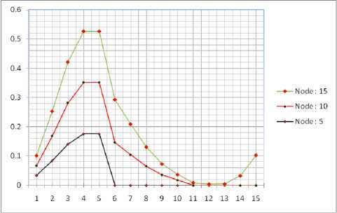
Fig. 11. The randomly distributed nodes deployment

• VI. Conclusion

In WSN, node clustering is very important in WSNs because it provides a topology control approach to reduce transmission overheads and exploit data aggregation among a large number of sensor nodes .Clustering mechanisms have been applied to sensor networks with hierarchical structures to enhance the network performance while reducing the necessary energy consumption. Clustering is a cross-cutting technique that can be used in nearly all layers of the protocol stack. The primary idea is to group nodes around a cluster head that is responsible for state maintenance and inter-cluster connectivity.