Collision-free Random Paths between Two Points

Published Online June 2020 in MECS

In the first phase of our work, we have developed a novel computer algorithm to generate random paths between two points in space [1]. A random path consists of a finite number of connected points that are generated randomly and satisfy the condition: L(P i P n ) < L(P i-1 P n ). Where L(P 1 P n ) is the length of the path between the two connected points P 1 and P n . The aim was to be able to generate paths between two points in real-time that cannot be predicted in advance. Our work applies to many fields such as education, economics, computer science, AI, military, industry, and other fields of applied sciences. In the second phase, we have developed an ontology that describes the domain of discourse. The aim was two folds; firstly, to provide an optimized generation of best points that are closer to the target point. Secondly, to provide sharable, reusable ontological objects that can be deployed to other projects [2].

We reinforced our solution by the initiation of several projects that have been designed using and extending our work. One problem that we have faced is the existence of obstacles in some cases between the starting point and the ending point. For example, in our work towards the automation of a navigation system for drones, we faced some obstacles like trees, no flying zones, buildings, among other obstacles. In this phase of our work, we have reworked the algorithm to generate random paths between two points P 0 (x 0 , y 0 ), P n (x n , y n ) with obstacles. Also, we have classified the generated paths based on given properties such as the longest path, shortest path, and paths with some given costs. The resulted algorithms were very encouraging and leading to the applicability of real-life cases. The following section presents related work. Section 3 discusses the structures and algorithm used in our work. In section 4, we provide a discussion on the assessment and evaluation of our work. The work is concluded in section 5, and future work is presented.

II.    Related Work

The generation of paths between two points is also called path planning, and increasingly being employed in the navigation of mobile robots and unmanned vehicles. Mobile robots are used in many automated environments such as servicing older adults, transferring goods in large factories, agriculture and farming, transportation, and military applications [3]. Researchers have worked on and proposed many algorithms for path planning in recent years. The task of generating free-collision, suitable paths in real-time is computationally challenging. Most early works reduced the problem into the two-dimensional grid, and transformed obstacles into blocked cells; graphsearching algorithms are then used on the resulted map to find suitable paths between the starting point and the target point [4, 5]. In many cases, Dijkstra’s algorithm, a well-known, greedy-based algorithm, has been used to find the shortest path between the starting point and the target point. The computation cost of Dijkstra's algorithm becomes O(N2), where N is the number of nodes. Less efficient pathfinding algorithms, in this case, may run as high as O(2n) [6, 7].     Early approaches became inefficient with more complex and dynamic environments. Other approaches utilize sensor-based models found in mobile robots equipped with cameras and other sensors. The movement is performed in a straight line toward the target point until an obstacle is confronted. Then, it tries to move around the edge of the obstacle, in an attempt of finding another suitable path. This approach works with unknown static environments. However, it becomes difficult when confronted with moving obstacles. Another problem is finding the optimal path when required. Later, researchers turned into evolutionary approaches such as Genetic Algorithms, Ant Colony Optimization, and Particle Swarm Optimization [8, 9, 10]. Evolutionary approaches model biological behavior found in insects, birds, and mammals. In recent years, hybrid models are being used where more than one approach is often combined to overcome their drawbacks. The system starts with the most straightforward approach, for example, moving towards the target point in a straight line. The system then steps up to another approach based on the current situation until reaching the target point. This is accomplished efficiently by the usage of hierarchal structures, where the higher level provides general directions (i.e., the location of the target point), and the lower level deals with obstacles, besides following the instructions from the higher level [11].

In our work, all points between the starting point and the target point are dynamically generated in real-time by a random function. We used a biased approach were each generated point is tested and validated base on some constraints, such as its location in relation with the target point and the existence of obstacles, which we will describe in detail in the following section.

In phase two of our work as described in [2], we have designed an Intelligence Consultation Unit (ICU) that guides the process of generating random paths between the starting point and the target point. We have used the

Object-Oriented Paradigm and UML (Unified Modeling Language) to build our model.

In this phase, we have extended our model to provide descriptions of which condition to consider based on the following criteria:

• 1.  L(P i P n ) < L(P i-1 P n ) , For i = 1, 2, …, n-1

• 2.  P i ∉ Z i , where Z i is the set of points inside an

• 3.    L(P i P i+1 ) does not pass through an obstacle.

obstacle.

Let P 0 and P n be two points. Initially, we generate a random displacement at the point P 0 ; the ICU considers the endpoint of that displacement is P 1 if it was acceptable. It means that our ICU decides if this displacement satisfies the above constraints and converges to P n . Otherwise, a new random displacement is generated. The process is repeated at point P 1 to obtain the next point P 2 , and so on until a point with a specific distance from P n is reached. When applying this scenario to mobile robots, points become the footsteps to follow one at a time. Once the robot reached a point, the remaining distance is re-evaluated, and a new decision that satisfies the above constraints are taken. The process of generating the paths is very fast and works well in complex and dynamic environments.

III.    The Generation of Random Paths with Obstacles

In this section, we present the main contribution of this paper. We have extended our work to handle the existence of obstacles in order to provide collision-free paths. We have built a UML model that defines the various concepts that describe the domain of discourse. We have used geometrical entities like points, lines, circles, and squares.

Our generated random paths are placed within circles that are centered in P n : c 1 , c 2 , …, c n-1 , which passes thru the points P 1 , P 2 , …, P n-1 respectively. Point P i may approach P n if it takes any position within circle c centered in P n with radius P i P n and satisfies the following constraints:

• 1.  L(P i P n ) < L(P i-1 P n ) , For i = 1, 2, …, n-1

• 2.  P i ∉ z i , where z i is the set of points inside an

• 3.    L(P i P i+1 ) does not pass through an obstacle.

obstacle.

The position of P i is generated randomly based on the following equations:

x += random(2*L+1) - L;           (1)

y += random(2*L+1) - L;           (2)

A random displacement is generated at point Pi(xi,yi) within a square with the length of sides equal to (2L), and point Pi+1 as the endpoint of that displacement if it was located within the circle ci. The generation process is repeated at Pi+1, and within the Circle ci+1 centered in Pn with radius Pi+1Pn to obtain new point P2. This iteration comes to a halt when reaching a point with a specific distance from Pn. This process will result in obtaining a set of points P1, P2… Pn, which satisfies the first constraint, and can also be written as the following:

L(P n-1 P n ) < L(P n-2 P n ) < . . . < L(P 1 P n ) < L(P 0 P n ) (3)

Circles and squares play an important role in directing the generated paths to reach the target point. The length of the side of the square limits the distance between the accepted points.

The second constraint guarantees that the generated point does not belong to the set of points falling inside an obstacle. Obstacles are transformed into geometrical shapes. Treating an obstacle as a geometrical entity allows us to compute the points that lay inside its boundaries; therefore, we can quickly check that line PiPi+1 does not pass through an obstacle. An acceptable shape we used in our work is a circle. The assumption that an obstacle falls inside the boundaries of a circle allows us to generate collision-free paths with low computational cost as will be shown below.

Figure 1 presents our extended higher-level model, which uses the object-oriented paradigm, where the ICU unit, the generated path, and all shapes that we use are instantiated objects. We begin by initializing the starting point P 0 , the ending point P n , L, and d. Then we create new objects for the path and for the ICU. The iteration starts with generating the first random point. The new point is then sent to the ICU unit to check for the constraints. If the point is accepted, we update our path, and a new random point is generated. We iterate through the process until the target point is reached.

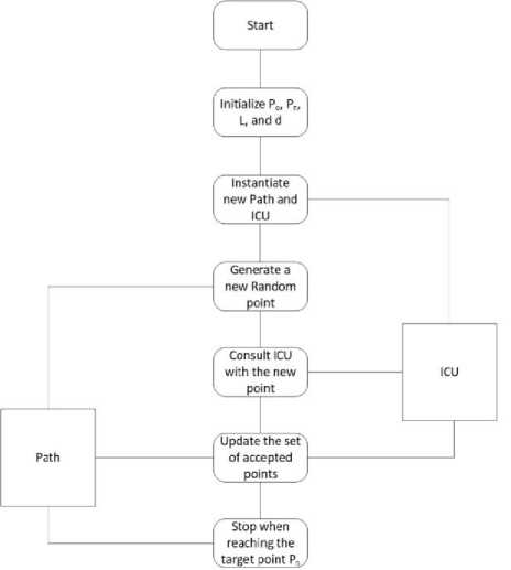
Fig.1. Path generation model

The ICU is a rule-based engine that is used to decide which points to accept based on certain thresholds that are explained previously.

Our extended algorithm consists of the following steps:

• 1.    Initialize x 0 , y 0 , x n , y n , L, d

• 2.    Let P(x, y) be current position, then x←x 0 , y←y 0

• 3.    Calculate distance L1(P, P n ) between P and P n

• 4.    Generate a random displacement at P(x, y) within a square centered in P and its side length is 2L,

• 5.    Calculate the new distance L2(P, P n )

• 6.    If (L2

so x ←x + Dx and y ←y +Dy

• a.    Link the points P and P 0

• b.    Rename the new position by P 0 (x 0 ←x,y 0 ←y)

• c.    Consider L1=L2

• 7.    If L2

• 8.    Go to step number 4

To test the algorithm, we have implemented a system in C-Sharp. In the implementation of the proposed algorithm, to ensure that our code is structured, we placed steps 4 to 7 inside a do-while loop, with the condition (L2>=d). For experimentations, the initial values for the starting point and the target point are entered by the user at the beginning of the run. In addition, the user may insert any number of obstacles and sets their sizes and locations.

We have performed our testing and evaluations in two sets; the first set was done without obstacles and the second set with obstacles.

• A.    Testing without obstacles

  In this set, we have tested the algorithm using 9 cases, where we generate random paths in groups of 10, 100, 1000, 10000, 20000, 40000, 60000, 80000, and 100000 iterations. We recorded all the results in table 1. Figure 2 shows the graphs of the generated random paths without obstacles for the first four cases.

We have chosen the locations for P0(x0,y0) to be (300, 300) and for Pn(xn,yn) to be (1000, 300) during all tests in this set. This is to ensure objectivity when performing the comparisons. In these experiments, we have used the Cartesian Plane with the point (0,0) located in the top left corner, and the units used are in pixels. Therefore, the distance between P0 and Pn is equal to 700, based on the following equation:

Distance ( P o , P_n ) = V ( X „ - X o )² + Y - Y o ) 2 (4)

We computed the length of each random path, in addition to the minimum, the maximum, and the average distance for each case as shown in table 1.

Table 1. Length Of Each Path With Different Iterations

Case	Number of Iterations	Length of Straight Path	Length of Min Generated Path	Length of Max Generated Path	Length of Average Generated Path
1	10	700	809	1339	1066
2	100	700	871	1403	1049
3	1000	700	803	1542	1056
4	10000	700	794	1536	1054
5	20000	700	780	1566	1055
6	40000	700	780	1592	1055
7	60000	700	761	1606	1056
8	80000	700	742	1627	1056
9	100000	700	733	1633	1055

The most important observation in this table is that the greater the number of iterations, the length of the shortest path is approaching the value of 700 which represents the straight path between P 0 and P n . Also, the length of the longest path is going above 1600.

Case 4

Case 1

Case 2

Case 3

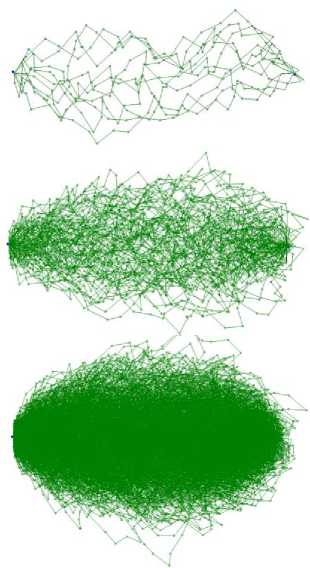
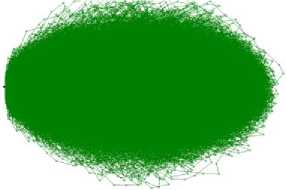
Fig.2. Four cases of random paths without obstacles

The plotted path in figure 3 represents the results with no obstacles, where we can also see the average with the higher number of iterations is converging to around the 1000 line, and the minimum distance, with the larger number of iterations, is approaching the 700 lines.

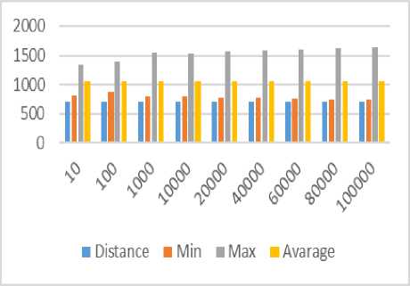
Fig.3. Results with no Obstacles

• B.    Testing with obstacles

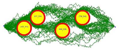
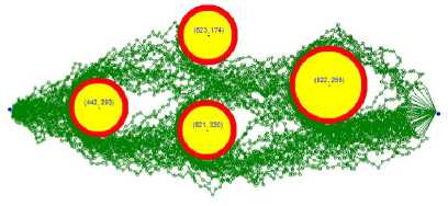
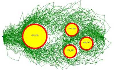
We have tested the algorithm using a different number of obstacles, sizes, and locations, and recorded all the results. Figure 4 shows 4 cases, where each case presents a set of obstacles and many generated paths, connecting the starting point with the target point. Obstacles are presented as yellow circles.

To ensure the generation of %100 collision-free paths, we have placed safe zones around each obstacle, which are shown in red. In theory, where well-defined mathematical principles are used, the safe zone can be eliminated. However, in real life with mobile objects, for example, robots, drones, and moving obstacles, a safe zone may become a lifesaver.

In the first two cases, we have set the distance between adjacent points to 10, while in the third and fourth cases, we have set the distance between adjacent points to 50. The generated paths in the first two cases are smoother, more focused, and shorter in comparison with the last two cases. In all cases, the generated paths converged to the target point, avoiding all obstacles. Moreover, the condensation of the paths, shown in a darker color, have shown that most paths favored the shortest path between the starting point and the target point. The time complexity of our algorithm is O(n), running one loop equal to the number of the generated points between the starting point and the target point. Most of the operations done in this algorithm is generating points, calculating distances, and deciding which one is closer to the target point that satisfies the constraints described above. The analysis of our algorithm is presented in detail in the next section.

We chose the same locations for P 0 (x 0 ,y 0 ) to be (300, 300) and for P n (x n ,y n ) to be (1000, 300) during all tests. The actual distance between P 0 and P n is also equal to 700.

We calculated the length of every edge and path for every case. The results are shown in Table 2. The maximum path length shown in the table is close to 1500, and the minimum is close to 1000, where the average is approximately 1170.

Case 1

Case 2

Case 3

Case 4

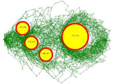
Fig.4. Four cases of random paths with obstacles

Table 1. Results obtained from the four cases

	Case 1	Case 2	Case 3	Case 4
Number of Paths	50	50	100	100
Starting Point	300,300	300,300	300,300	300,300
Target Point	1000,300	1000,300	1000,300	1000,300
L(P i P i+1 )	10	10	50	50
Actual length	700	700	700	700
Shortest path	943	919	880	892
Longest path	1164	1106	1469	1396
Average Length	1019	1004	1118	1102

We took one case this time and tested the algorithm again with the distance between two points is 50. This time we randomly generated paths in groups of 1, 10, 100, 1000, and 10000 iterations. We computed the length of each random path, in addition to the average, the minimum, and the maximum distance for each group as shown in Table 3.

Table 2. Length of each path with different iterations

Number of Iterations	Length of path	Average	Max	Min
1	700	1013	1013	1013
10	700	995	1131	884
100	700	1069	1308	878
1000	700	1075	1441	825
10000	700	1074	1507	789

Looking at table 3, we see that the average stayed in the range of 995 and 1075, while the minimum distance ranged from 789 to 1013. The plotted path in figure 5

presents our findings, where we can see the average stayed around 1000, and the minimum distance, with the larger number of iterations, is converging towards the distance of 700.

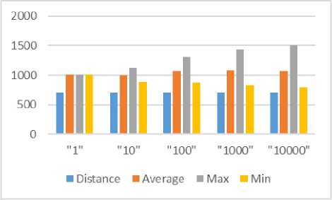
Fig.5. Results with Obstacles

IV.    Discussion and Evaluation

The main objective of this work is the addition of obstacles and the generation of free-collision random paths. We have tested the algorithm with many cases; each has a different set of constraints with a variety of obstacles. Our obstacles have different sizes and locations. Moreover, we have generated random paths up to one hundred thousand paths, covering many possibilities. In all cases, the generated paths converged to the target point, avoiding all obstacles. Moreover, tests have shown that paths favored the average-length path between the starting point and the target point.

From the literature review shown in section 1, the time complexity of all the algorithms that we have reviewed ranged from O(n2) to O(2n). The time complexity of our algorithm is O(n), running one loop equal to the number of the generated points between the starting point and the target point. Most of the operations done in this algorithm are generating points, calculating distances, and deciding which one is closer to the target point that satisfies the constraints described above. The analysis of our algorithm is follows:

Steps of the Algorithm          Running Time

Initialize x0, y0, xn, yn, L, d

Let P(x, y) be current position, then x←x0, y←y0

Calculate distance L1(P, Pn) between

P and P n

LOOP (while L2> d) BEGIN:

Generate random displacement at P(x,       3n + C 3

y) within square centered in P and side length is 2L, so x ←x + Dx, y ←y +Dy

Calculate the new distance L2(P, P n )         ^{n + C4}

If (L2

• a.    Link the points P and P0

• b.    Rename the new position by P0(x0←x,y0←y)

END OF LOOP

T(n) 7n + C

As presented above, the sum of all constants C0 to C5 is equal to C, a constant. Thus, the time complexity of our novel algorithm yields to O(n).

V.    Conclusion and Future Work

We have proposed and implemented an algorithm, described in section 2, for generating collision-free random paths between two points (P0, Pn). We have tested the algorithm under all possible constraints, and the generated paths were able to converge to the target point avoiding all obstacles, which have different sizes and locations. The algorithm is very fast, with time complexity of O(n).

This work can be applied in many cases. During the second phase of our work, as described in [2], we have initiated several projects utilizing the algorithm. Extending the work to deal with obstacles was very helpful in solving problems faced us in some of these projects, as described in the following subsections.

• A.    Towards the Automation of Drone Navigation Systems

Unmanned aircraft (Drones) are becoming very popular these days. This is due to their low cost and the various applications they provide for humanity in many fields like farming, industry, transporting products, research, and military.

Most drones today use pilot-controlled navigation systems. Current technologies for automating the drone navigation systems is still in its infantry stages and open for research [12, 18, 19, 20].

Probably, one of the most faced challenges, in the task of automating the navigation of drones is dealing with obstacles such as buildings, trees, and other objects. This becomes much harder with moving obstacles, such as vehicles, and other drones. Planning such paths in a complex and dynamic environment becomes computationally very costly.

Over the last few years, due to its low cost and low risk of casualties, many countries around the world are utilizing drones in their military and civil operations. While it is easy to remotely pilot a single drone, controlling many drones while conducting various tasks becomes a major objective.

Current-generation drones face the limitations of flying at low altitudes and slow speed compared to manned aircraft. In hostile zones, flying drones from one point to another in straight lines are vulnerable to anti-air defense systems and therefore are easy targets.

The generation of random paths between two points in real-time, which cannot be predicted in advance, can be of great value to flying drones. This method would greatly minimize the loss of drones over disputed regions.

Due to the limitations of the current-generation drones, most countries are using them for surveillance purposes only.

To the authors’ knowledge, all current-generation drones are remotely piloted drones. While some developed counties are advancing the state-of-the-art drone technology in many directions, the development of self-piloted drones is still in its infant stage.

This research can be valuable work in this direction. We are applying our research findings towards the automation of drone navigation systems.

• B.    Crawling the World-Wide-Web

The World-Wide-Web is a huge dynamic digraph. Vertices in the graph are webpages, where each may contain textual data, images, and other multimedia elements. Hyperlinks are the edges that connect webpages together. Search engines use crawlers that traverse the web collecting and processing all types of data. Crawlers use breadth-first graph traversal algorithm to collect data and store it in databases.

Is it possible to crawl the web in random order? What kind of results may we get? Can we consider unwanted webpages as obstacles? How can we set up a starting webpage and a target webpage within this large dynamic graph?

These are some questions that we are working on in this project. One problem we are facing is dealing with geometrical shapes like circles and squares, which we have used to move closer to the target point. In this research, we are using costs instead, which are generated from some properties of the webpages.

Some scholars are using random walk theories to visualize subsets of the web and collect information in order to study web properties. Crawling the web in random order is an unbiased process, while our algorithm is biased because we must converge to the target point. Random walk models have been used in biology, physics, ecology, medicine, computer science, and other scientific disciplines [15, 16, 17].