Comparative Analysis of LSTM Variants for Stock Price Forecasting on NSE India: GRU's Dominance and Enhancements

The forecasting of future values in the financial domain, particularly concerning stock values, through time series analysis, is considered a critical and complex task. A complex and dynamic system, the stock market, reflects the collective behavior and sentiment of investors, being influenced by a multitude of factors ranging from economic indicators to geopolitical events. Its inherent unpredictability presents a significant challenge for investors, traders, and researchers seeking to forecast future price movements. Traditional financial models, such as the Efficient Market Hypothesis (EMH) and fundamental analysis, are provided with valuable frameworks for understanding market dynamics. However, they are often found to struggle in accounting for the non-linear relationships and sudden shifts in market sentiment that characterize real-world financial data.

Over the years, various approaches to forecasting stock market movements have been explored by researchers and practitioners, ranging from fundamental analysis and technical analysis to quantitative modeling and machine learning algorithms. Among these approaches, statistical methods occupy a central position, leveraging mathematical and computational techniques to analyze historical data and uncover patterns that may inform future trends. Statistical methods offer a systematic framework for understanding the underlying dynamics of financial markets and extracting actionable insights from vast amounts of historical data. Time series analysis, for instance, enables researchers to model and forecast the temporal dependencies inherent in stock price data, while regression analysis allows for the identification of relationships between stock prices and relevant predictors. Time series analysis is a fundamental statistical technique used to model and forecast sequential data points collected over time. In the context of stock market prediction, time series analysis enables researchers to capture the temporal dependencies and inherent patterns in historical price data. One of the most widely used time series models is the Autoregressive Integrated Moving Average (ARIMA) model, which incorporates autoregressive (AR), differencing (I), and moving average (MA) components to model stationary time series data. ARIMA models can be extended to seasonal time series data using Seasonal ARIMA(SARIMA) framework, which incorporates seasonal differencing and seasonal autoregressive and moving average terms. Additionally, the Generalized Autoregressive Conditional Heteroskedasticity (GARCH) model is frequently employed to capture volatility clustering and time-varying volatility patterns in financial time series data. Regression analysis is another powerful statistical technique used in stock market prediction to identify relationships between independent variables (predictors) and a dependent variable (stock prices). Linear regression is a simple yet effective method for modeling linear relationships between variables, wherein the coefficients represent the strength and direction of the relationships. More advanced regression techniques, such as Ridge regression and LASSO regression, are used to address multicollinearity and overfitting issues by introducing regularization penalties on the regression coefficients. Regression analysis can be extended to time series data using autoregressive distributed lag (ARDL) models, which incorporate lagged values of predictors to account for temporal dependencies.

In recent years, a new paradigm for analyzing and predicting stock market trends has been offered by the advent of machine learning. Machine learning algorithms, capable of processing vast amounts of data and identifying complex patterns, hold the potential to augment traditional financial models and improve prediction accuracy. By leveraging historical market data, along with a diverse set of features encompassing technical indicators, macroeconomic variables, and even sentiment analysis from news articles and social media, machine learning algorithms can uncover hidden relationships and provide valuable insights into future market movements. The application of machine learning in stock market prediction has garnered significant attention from both academia and industry. Various machine learning techniques, including regression models, decision trees, support vector machines, neural networks, and ensemble methods, have been explored by researchers to develop predictive models capable of forecasting stock prices with varying degrees of accuracy. Moreover, advancements in computational power, data availability, and algorithmic sophistication have further fueled the adoption of machine learning in financial markets. Despite the promising potential of machine learning algorithms, challenges such as data quality, feature selection, model interpretability, and market volatility pose significant hurdles to their widespread adoption. Moreover, the inherently stochastic nature of financial markets means that even the most sophisticated predictive models may encounter difficulty in accurately forecasting market movements over extended time horizons.

Nevertheless, the pursuit of accurate stock market prediction remains a compelling endeavor with far- reaching implications for investors, financial institutions, and policymakers. This research paper aims to contribute to this ongoing discourse by exploring the application of machine learning algorithms in stock market prediction, evaluating their efficacy, and identifying avenues for future research and development. By combining insights from both finance and machine learning domains, this study seeks to enhance our understanding of financial markets and facilitate more informed decision-making in the realm of investment and trading. Robust models [1-3] capable of capturing the intricate dynamics inherent in the ever- fluctuating [4-5] stock market is sought after by investors, analysts, and researchers alike.

In the pursuit of correct forecasting, the Long- and Short-Term Memory (LSTM) architecture has long been considered the go-to choose, standing as a stalwart in time series forecasting. The investigation takes place within the context of a substantial body of literature endorsing LSTM as the preferred model [6-9] for time series prediction. LSTM's capacity to apprehend extended relationships over time [10-11] and intricate behaviors [12] in sequential data has rendered it a cornerstone in the arsenal of predictive analytics within the financial sector. As financial markets, and particularly the NSE (National Stock Exchange) India [13-14], continue to evolve, the demand for advanced and adaptive models becomes increasingly imperative. As the financial landscape evolves and datasets become more diverse and complex, researchers and practitioners continually sought ways to enhance LSTM's capabilities [15-16].

This has prompted the emergence of diverse advancements in LSTM variants, each tailored to specific characteristics of the data. Bidirectional LSTMs, stacked LSTMs, Gated Recurrent Unit and Drop-out LSTM are among the advancements that have targeted to refine the capability of the model in handling different types of temporal dependencies [17-18] and capturing nuanced patterns [19-20] in financial time series. Motivated by the diversity of stocks within NSE India, it was hypothesized that certain LSTM variants could be tailored to align with the unique characteristics and behaviors associated with specific sectors. This assumption was grounded in the belief that a nuanced approach, accounting for sector-specific dynamics [21-24], could potentially unlock superior predictive capabilities. The initial premise was to recommend specific LSTM variants for each sector, subsequently enhancing their performance through a sector-centric lens [25-26].

The primary research question driving this study is whether specific LSTM variants are better suited for predicting stock prices in particular sectors due to their architectural differences. This forms our first research objective. If the hypothesis is not supported and no such correlation is found, the next objective will be to identify which LSTM variant performs the best overall across all sectors. Additionally, we aim to explore whether this dominant variant has limitations, and based on these findings, we will develop appropriate techniques to enhance prediction accuracy of this dominant variant.

2.    Related Works

Strong forecasting techniques for well-informed choices are necessitated by financial markets, which are characterized by their intricate dynamics and constant fluctuations. Significant advancements in time series prediction, a vital aspect of financial forecasting, have been witnessed, particularly in the context of India’s National Stock Exchange (NSE). The current information of research on time series prediction is critically examined in this literature review, with a focus on the utilization of Long and Short Term Memory (LSTM) models and their enhancements to unravel the intricacies of the NSE India stock market.

A noticeable transformation in the landscape of stock market forecasting was undergone prior to the year 2000, marked by the application of diverse machine learning methods [27-31]. As technology advanced, the search for more accurate and efficient forecasting methods was intensified. In this evolving domain, the emergence of Long and Short Term Memory (LSTM) after 2000 was found to be a pivotal development [32-34]. Superior capabilities in identifying long time dependencies [35,36] and trends not only in other time series domains but also within stock market data have been demonstrated by LSTM, a recurrent type of neural network (RNN). Its effectiveness in handling sequential information and understanding complex relationships among various market factors set it apart from traditional machine learning approaches.

The superiority of LSTM models is clearly evident in the extensive literature review, as numerous studies highlight their consistent performance and widespread adoption in time series forecasting tasks. Han, Zhongyang, Jun Zhao, Henry Leung, King Fai Ma, and Wei Wang [37] conducted a comprehensive review of deep learning models for time series prediction, focusing on six distinct methods. Their analysis revealed that LSTM and hybrid models exhibited greater stability in the implemented experiments compared to other models. In a related study, Tang, Yajiao, Zhenyu Song, Yulin Zhu, Huaiyu Yuan, Maozhang Hou, Junkai Ji, Cheng Tang, and Jianqiang Li [38] carried out a survey on machine learning models for financial time series forecasting. Over a period of 10 years, they found LSTM to be utilized in 80 research articles, significantly surpassing the 42 articles for the next widely used machine learning model. LSTM's accuracy and popularity contributed to it being the most cited model, with 368 citations. Similarly, Rahimzad, Maryam, Alireza Moghaddam Nia, Hosam Zolfonoon, Jaber Soltani, Ali Danandeh Mehr, and Hyun-Han Kwon [39] conducted a performance comparison between an LSTM-based deep learning model and conventional machine learning algorithms for streamflow forecasting. They found that the LSTM model proposed for daily streamflow prediction demonstrated superior performance among all the models tested.

LSTM and its hybrid approaches have consistently proven to be the most effective models across various time series datasets [40-42]. A structure employing the LSTM (Long and Short Term Memory) paradigm and the business's net expansion computation algorithm for the scrutiny and anticipation of a company's forthcoming growth is advocated by Maji, Ghosh, and Debnath [43]. An enhanced prognostic framework constructed on the long and short term memory (LSTM) structure to autonomously retrieve historical stock values from the internet within a designated time frame is introduced by Mehtab, Sen, and Mondal [44]. Furthermore, future prices for a specified forecasting duration are anticipated and forthcoming stock prices are projected by the framework. The Long and Short Term Memory (LSTM) network is suggested by Chatterjee and Salimath [45] for determining stock movements. Additionally, a comparative examination and analysis of four distinct network structures are offered by them. Historical data provided openly by the National Stock Exchange (NSE) of India is retrieved. Utilizing recurrent neural networks (RNN) with long and short term memory (LSTM), Mohan and Naik [46] forecast future stock returns by prioritizing recent over historical stock information. To prevent overfitting, recurrent dropout is applied to RNN layers. Data from the National Stock Exchange, India (NSE), is used for experimentation, revealing the superior performance of the proposed RNN with LSTM model compared to a feed-forward artificial neural network. A dataset derived from the Indian stock market is utilized by Jha and Yadav[47], constructing an LSTM model accordingly. Subsequently, optimization ensues through contrasting stateless and stateful models, alongside fine-tuning the quantity of hidden layers. A methodology grounded in an impartial framework is introduced by Vinaykumar and Selvin [48]. Rather than conforming the data to a particular model, they discern the inherent dynamics within the dataset employing deep learning structures. Employing a sliding window methodology, short-term future values are forecasted. An advanced Deep Learning-driven Long and Short Term Memory (LSTM) Algorithm is advanced by Gupta and Sisodiya [49]. The National Stock Exchange (NSE) of India furnishes a decade's worth of past stock price records for the NIFTY 50 index. Following normalization, this dataset is employed for both model training and testing. The outcomes of the proposed model exhibit considerable promise, achieving an accuracy rate of 83.88 percent. A model that surveilled stock data of Samsung Electronics and news updates via textual analysis, unveiling a prognostic framework by showcasing the scrutinized outcomes, is introduced by Sunghyuck Hong [50]. Eight regression algorithms employing the training dataset containing NIFTY 50 index data from December 29, 2014, to December 28, 2018, are constructed by Sen, Mehtab, and Dutta [51]. Utilizing these regressive models, forecasts are made for the opening values of NIFTY 50 spanning from December 31, 2018, to July 31, 2020. Subsequently, the predictive capability of their framework for forecasting is enhanced by developing four regression models based on deep learning, employing long and short term memory (LSTM) networks, accompanied by an innovative method of walk-forward validation. Long and Short Term Memory (LSTM) is employed by Priya and Himanshu [52] to prognosticate forthcoming stock market prices. LSTM concentrates on prophesying stock prices by leveraging past day's closing figures, and it is being utilized to anticipate the TATA GLOBAL stock's trajectory by incorporating multifaceted input parameters to assess its predictive efficacy on the stock's temporal data. A model utilizing investor sentiment for stock forecasting is proposed by Jin and Liu [53]. They advocate for systematically disassembling the intricate sequence of stock prices through the utilization of empirical modal decomposition (EMD). Additionally, they suggest refining it further with Long and Short Term Memory (LSTM) and employing an attention structure to concentrate more on pivotal data points. A recent study conducted by Das and Ghosh [54], which utilized four deep learning networks along with LSTM (Long Short-Term Memory) on day-wise closing prices from both the National Stock Exchange (NSE) of India and the New York Stock Exchange (NYSE), has significant implications for stock market forecasting. Their comparative analysis against the ARIMA (Autoregressive Integrated Moving Average) model highlighted the superior ability of neural networks, demonstrating their capability in identifying trends in the stock market. A collaborative approach that integrates deep learning principles to aid in stock selection and optimal portfolio construction using predictive techniques alongside the mean-variance (MV) model is proposed by Jha and Priya Singh [55]. In their initial phase, they introduce the CNN-LSTM model, which merges the benefits of both the convolutional neural network (CNN) and the long and short term memory network (LSTM). This model effectively amalgamates learning in sequence combined with feature selection to capture temporal variations in data.

Advanced variants of Long and Short Term Memory (LSTM) networks are increasingly being deployed in the realm of stock market prediction. These sophisticated LSTM models, such as stacked LSTMs, bidirectional LSTMs, and attention-based LSTMs, offer increased ability in determining intricate structures and relationships within time series data in the finance domain. By leveraging these advanced architectures, analysts aim to enhance the precision and resilience of their stock market forecasting models, thereby enabling improved decision making through knowledge inside the ever-changing and erratic financial markets [56-57]. Following an extensive literature review, the Long Short-Term Memory (LSTM) model has emerged as the most viable option for forecasting stock market movements. Various advanced iterations of LSTM have been explored by researchers to enhance predictive accuracy. This paper aims to contribute to the field by constructing a prediction model utilizing these sophisticated LSTM variants.

3.    Modelling Approach

The advanced variants of LSTM models have been explored by only a limited number of researchers. Our method was prompted by this scarcity of investigation, with the aim of achieving superior performance. LSTM, renowned for its exceptional results in time series prediction compared to other algorithms, served as the impetus for our exploration.

• 3.1.    A Brief Overview of LSTM Variants

Long Short-Term Memory (LSTM) networks have evolved with advanced variants being catered to diverse needs in sequential data modeling. Simplified architectures with comparable performance are offered by variants such as Gated Recurrent Units (GRUs), while the memory cell of LSTM is enhanced by peephole connections incorporating information from the cell state into the gating mechanism. Furthermore, attention- based mechanisms enable LSTM networks to focus on relevant information within sequences, facilitating tasks like machine translation and sentiment analysis. Additionally, overfitting is mitigated by techniques like zone out and variational dropout, ensuring robustness in training large-scale LSTM models. The capability to capture long-term dependencies and tackle complex sequential data analysis tasks across various domains is collectively enhanced by these advanced variants. Some variants were tested out, assessing their effectiveness in forecasting stock market prices based on features that appeared promising. The selected variants include Bidirectional LSTM, stacked LSTM, dropout mechanism LSTM, and Gated Recurrent Unit (GRU).

• A.    Basic LSTM

The LSTM architecture is primarily composed of three gates: input, output, and forget gates, as well as a memory cell that has the capacity to store data over time. These gates can be used by LSTMs to retain or discard information from previous time steps. The transmission of data into and out of the memory cell is controlled by these gates. The appropriate amount of newly acquired data to be stored in a cell in the memory is established by the input gate.

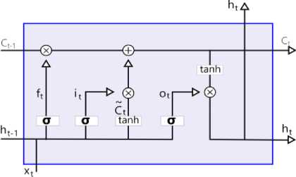
Fig.1. LSTM architecture

The input gate establishes the appropriate amount of newly acquired data to be stored in a cell in the memory.

t, = ^ (W i • [ h t - 1 , X t ] + bl )

The forget gate determines which data from the cell should be ignored.

f, = vW •[h(t-1),xt] + bf )

Depending on the state of the cell, the output gate determines what information to output.

ot = CWo ■[h(t-1), xt ] + bo )

The forget and input gates use cell state to update the long-time memory of the memory cell.

ct = fc-i + iq

The LSTM cell's output, or hidden state, is a filtered representation of the cell state.

h_t = o_t tanh( c_t )

• B.    Bidirectional LSTM

A Bidirectional Long and Short Term Memory (LSTM) represents a recurrent neural network (RNN) architecture incorporating LSTM units. Its bidirectional nature signifies its ability to analyze input sequences in forward as well as backward sides. The network accesses information from both past and future states at each time step, which proves advantageous for various sequence modeling tasks. The functioning of a Bidirectional LSTM can be outlined as follows:

• •    Forward Propagation: Like a conventional LSTM, the input sequence undergoes processing from start to finish. At every step, hidden states are calculated using the present input and the preceding hidden state.

• •    Backward Propagation: Contrarily, the input sequence is traversed in reverse, from the end to the beginning. This mechanism enables the network to capture insights from future states of the sequence.

• •    Combining Outputs: The outputs getting from the forward passes and backward passes are typically combined in some way. This could involve concatenating them, adding them together, or using some other operation to merge the information.

Let ht forward and ht backward show, for the forward and reverse LSTMs, the hidden states at time step t.

The output of the Bidirectional LSTM at time step t is:

( forward )

hi = L ^h ( t )

( backward )

Bidirectional LSTMs are frequently employed in NLP domain uses such as recognizing named entities, identification of sentiment, machine translation, and audio recognition, where meaning from both past and future portions of a sequence is significant.

• C.    Stacked LSTM

A recurrent neural network (RNN) architecture comprising multiple LSTM layers arranged vertically is represented by a stacked Long and Short Term Memory (LSTM) configuration. Enduring relationships within sequential datasets are excelled in by these LSTM networks, a subtype of RNNs. The operation of a stacked LSTM is unfolded as follows. Sequential data, which may include time-series information, textual data, audio signals, etc., is analyzed by stacked LSTM models, analogous to other RNNs. Within a stacked LSTM design, several LSTM layers are organized in succession, and each layer processes the input sequence and forwards its output to the subsequent layer. The input sequence is received by the initial layer, and outputs from preceding layers are received by subsequent parts. A hidden state and a cell state are maintained by each LSTM layer, preserving information from earlier time steps, and these states facilitate learning enduring dependencies by selectively retaining or discarding information.

By stacking multiple LSTM layers, hierarchical understandings of the input are acquired by the network, wherein lower layers capture rudimentary features and temporal patterns, while higher layers extract abstract and intricate representations. Back propagation through time (BPTT), an advancement of back propagation tailored for sequences, trains stacked LSTM networks during training, wherein the model computes its weight values to decrease deviations between predicted and actual outputs. Success across diverse domains such as NLP, audio recognition, and time series forecasting has been found by stacked LSTM configurations, owing to their adeptness in capturing prolonged dependencies, which significantly contributes to their performance. In essence, the network is empowered to discern intricate patterns and representations within sequential data by the stratification of LSTM layers, thereby enhancing its predictive capabilities. Nevertheless, this enhancement comes at the cost of increased computational complexity.

• D.    Drop-out based LSTM

Dropout is utilized as a regularization strategy widely in neural networks to counteract overfitting. In the realm of traditional feedforward neural networks, dropout involves the random nullification of a portion of neurons' outputs during training, thereby thwarting the tendency of neurons to co-adapt. Similarly, dropouts can be integrated into LSTM networks by randomly zeroing a fraction of the hidden units' outputs. The implementation of dropout within LSTM networks aids in mitigating overfitting by introducing variability into the network and diminishing the reliance of neurons on specific input features. More resilient representations of the input data are fostered by this regularization approach, thus enhancing the network's capacity for generalization to unseen instances. Dropout in LSTM networks can be applied to different components of the network, such as input-to-hidden connections, recurrent connections, or hidden- to-output connections. By applying dropout to different parts of the network, it becomes possible to control the amount of noise injected into the model and prevent over fitting effectively.

• E.    Gated Recurrent Unit (GRU)

The architecture of the GRU comprises a network of recurring units, each intended to maintain and update a hidden state as sequential input data is processed. The following components are involved in the basic structure of a GRU unit.

Z t = v (W_zX t + Uh - 1 + b z )

r = a (W_rX t + U_rh t - 1 + b_r )

yt = tanhWhXt + Uh (ht-I /;) + bh ht = ztht-i + (1 - zt) y

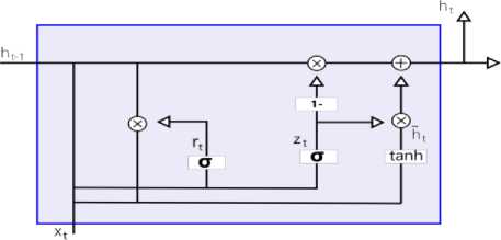
Fig.2. GRU architecture

The hidden state, at every time step, reflects the network's memory. It serves as a memory cell, capturing relevant information from previous inputs. The input gate, designed for inputting, determines which parts of the input data should be saved in the hidden state. It considers the current data to be inputted and the hidden last state. The update gate decides the amount of the prior hidden state that has to be kept for this time step. It controls data flow from the earlier hidden state to the active hidden state. One notable feature of GRU is its simplified structure compared to LSTM. It has fewer parameters, making it computationally more efficient and faster to train. The functionalities of the inputting and forgetting gates in LSTM are combined into a combined gate in GRU to update the data. This reduces the complexity of the architecture. GRU is specifically capable of capturing short-term relationships in sequential data. It has been observed to perform well in tasks where remembering recent information is quite important. In summary, the GRU architecture presents a streamlined version of the LSTM, demonstrating efficiency in training and good performance, especially in scenarios where capturing short-term dependencies is essential. Contrary to our initial hypothesis, GRU was consistently outperformed by LSTM across all sectors. This unexpected outcome prompted a thorough investigation into the limitations of GRU compared to LSTM, focusing on its struggles with capturing long-term dependencies.

• 3.2.    Model Design

• 3.3.    Dataset Selection and Pre-processing

In our methodology, a meticulous journey through the complexities of the NSE India stock market was embarked upon, with LSTM (Long Short-Term Memory) model variations being employed to delve into the nuanced behaviors and characteristics inherent in various sectors. Our primary objective was to discern whether LSTM variants could be fine-tuned to harmonize with the distinctive traits exhibited by specific sectors within the market landscape. This initial phase of assessment was crucial, as it served as the bedrock upon which tailored predictive models that encapsulate sector-specific dynamics could be built.

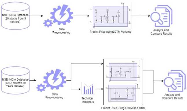
Fig.3. Model design

To our surprise, contrary to our initial hypothesis, the GRU (Gated Recurrent Unit) model was consistently outshone by LSTM across all sectors. This unexpected outcome prompted a deep dive into the limitations of the GRU architecture for large datasets, if any. While GRU's superior performance underscored its efficacy as a predictive tool, it also unveiled certain constraints that necessitated further scrutiny. Understanding these limitations became imperative for ensuring the robustness and reliability of our predictive models in real-world applications. In the subsequent phase of our study, efforts were made to address these identified limitations by integrating technical indicators into the dataset. Technical indicators play a pivotal role in gauging market trends and patterns, offering valuable insights into the underlying dynamics of stock price movements. By incorporating these indicators, the aim was to enrich the predictive capabilities of our models, augmenting their capacity to capture subtle nuances and anticipate market behavior more accurately.

Upon completion of model development and refinement, the performance of our proposed model was meticulously evaluated against the baseline GRU model. This validation step was essential for corroborating the efficacy and superiority of our approach, ensuring that the proposed model not only addressed the limitations of GRU but also delivered tangible improvements in predictive accuracy and reliability. By subjecting our model to rigorous validation procedures, efforts were made to instill confidence in its efficacy and applicability across diverse market scenarios, thereby enhancing its utility as a valuable tool for informed decision-making in the realm of stock market investments.

The selection of a dataset for stock market price prediction research depends on the specific objectives of the modeling and the characteristics of the market being analyzed. The NSE India dataset is ideal for stock price prediction in emerging markets, as it reflects sectors like IT, banking, and energy, which are highly representative of the Asian economy. Given the unique regulatory environments, volatility, and liquidity in such markets, stock movements can vary significantly across sectors. Using advanced variants of LSTM models, which offer architectural flexibility, allows for sector-specific forecasting. This dataset provides an excellent opportunity to study sector dynamics in a growing and volatile market, where different models can be tailored to specific industries.

Historical stock price data from the NSE India was collected for a diverse set of stocks representing five distinct sectors: Pharma, Automobile, Energy and Gas, and Information Technology. Four leading stocks from each sector within the NSE India stock market were chosen to ensure a comprehensive analysis of the models' execution. The data collection included daily closing prices, trading volumes, and other relevant metrics. A time frame spanning 5 years was considered to ensure consistency.

Table 1. Stock selection across diverse sectors

Automobile	Banking	Oil and Gas	Pharma	IT
Bajaj Auto	Axis	BPCL	Cipla	HCL
Eicher motors	HDFC	IOCL	Dr. Reddy	Infosys
Hero Motocorp	icici	ONGC	LUPIN	TCS
TATA Motors	SBI	Reliance	Sun pharma	Wipro

The dataset was standardized during data pre-processing to address variations in scale among different stocks. Additionally, missing data and outliers were handled using appropriate techniques. In assessing the performance disparities between Gated Recurrent Unit (GRU) and Long Short- Term Memory (LSTM) models, datasets centered on TATA MOTORS stock was utilized. The comparative analysis involved a shorter dataset spanning five years and a longer dataset extending over a decade. Furthermore, to overcome the inherent limitations of the GRU model, particularly when confronted with extensive datasets, various technical indicators were incorporated for comprehensive evaluation over a 20-year period. The incorporation of Moving Averages (MA), Moving Average Convergence Divergence (MACD), Relative Strength Index (RSI), and Bollinger Bands enhanced the analytical depth and accuracy of the study. These indicators are generated using ‘TA’ library. Missing data was handled using the nan_to_num function from the yfinance module.

4.    Experiments Setting and Results

A sequence of experiments was meticulously designed to follow our objectives. An expansive examination spanning diverse sectors was commenced, and stocks were subjected to rigorous analysis, employing a plethora of LSTM variations. This initial experiment, conducted over a span of five years, served as a foundational benchmarking exercise. Upon meticulous evaluation, the GRU model notably emerged as the most promising contender, demonstrating superior performance metrics across all variants considered for the stock data spanning a five-year period. This comparative analysis not only reinforced the prowess of the GRU model but also laid the groundwork for subsequent endeavors. With a solid foundation established, the scope of the investigation was sought to be broadened by extending the analysis to a more extensive dataset encompassing two decades of stock market dynamics. However, certain inherent limitations within the GRU model were brought to light by this expansion, particularly when confronted with larger datasets characterized by increased complexities. Undeterred by these challenges, the third experiment was meticulously crafted to address and mitigate these shortcomings. In this third iteration, the endeavor was made to augment the predictive capabilities of the GRU model by integrating additional technical indicators into the analytical framework.

Here are the detailed configurations and steps for the LSTM variants, GRU, and how technical indicators were incorporated into the models. GRU and LSTM variants were used with a multi-layered architecture. A two-layer setup was implemented, with each layer consisting of 100 units (neurons). A dropout of 20% was applied after each GRU/LSTM layer to prevent overfitting, and a fully connected (Dense) layer was added to map the output to the final prediction of the closing stock price The hyperparameters for both models were selected through Random Search, exploring layers between 1 to 3, units per layer between 50 and 200, learning rates from 0.0001 to 0.01, batch sizes of 32, 64, and 128, and the Adam optimizer with early stopping based on validation loss. Various look-back periods, such as 10, 20, and 30 days, were tested, and the 20-day period provided the best performance. The models were trained for up to 100 epochs with early stopping, using a batch size of 64, Mean Squared Error (MSE) as the loss function, and the Adam optimizer with an initial learning rate of 0.001. The software stack included Python (v3.8), TensorFlow (v2.10), Keras, Pandas, NumPy, and Matplotlib, and the data was sourced from Yahoo Finance via yfinance. Following these steps, researchers should be able to replicate the results effectively.

Table 2. Parameters setup

Parameter	Value
Look Back Period	20
Batch Size	64
Epochs	100
Units in 1st Layer	100
Number of Layers	2
Units in 2nd Layer	100
Learning Rate	0.001
Optimizer	Adam
Loss Function	Mean Squared Error (MSE)
Data Split	67% Training, 33% Testing
Activation Function	tanh

Technical indicators such as Moving Average (MA), Moving Average Convergence Divergence (MACD), Relative Strength Index (RSI), and Bollinger Bands were incorporated as additional features. These were appended to the stock price dataset along with open, high, low and closing price, calculated using a 14-day look-back window, and normalized using MinMaxScaler for consistent processing by the neural network. The selection of technical indicators was done according to the limitations identified in the dominant variant, i.e., GRU. This limitation guided the choice of technical indicators, ensuring that the selected indicators would complement the model's strengths while addressing its weaknesses. These choices and their rationale are discussed in detail in Chapter 4.3.

• 4.1.    Use of LSTM Variants for Various Sectors

• 4.2.    Performance Evaluation of Winner Variant (GRU) for Complex Dataset

  It was pointed out that GRU employs fewer gates than LSTM, potentially leading to faster learning processes in time series forecasting. Fewer gates make it computationally efficient while retaining key features for learning sequential patterns. They mitigate the vanishing gradient problem more effectively and perform well with smaller datasets or when long-term dependencies aren't as critical. However, before settling on GRU, it is essential to thoroughly investigate its performance. The size of the dataset is the first consideration. Previous experiments likely employed a small dataset, and it is crucial to assess whether GRU can excel with limited data. However, it is acknowledged that relying solely on small datasets might not provide a comprehensive understanding of the model's capabilities. Thus, the proposal is to extend the analysis to larger datasets as well to test for complexity associated with large datasets. The inclusion of a larger dataset introduces complexities and unpredicted patterns that might not be evident in smaller datasets. This expanded scope allows researchers to evaluate how well such challenges are handled by GRU. Furthermore, insights are offered into whether GRU requires refinement to effectively manage the intricacies of larger datasets. To illustrate, the utilization of datasets from TATA Motors spanning 20 years duration is proposed starting from January 2001. By examining this large dataset GRU's performance across a spectrum of complexities and durations can be assessed. The importance is emphasized not only on assessing the model's performance with a large dataset but also on exploring its scalability and adaptability to long dependencies, more intricate datasets. This approach

The results were embarked upon with an ambitious hypothesis: that certain Long Short-Term Memory (LSTM) variants might be outshone by others in analyzing specific sectors within the NSE India stock market, owing to their unique features. With this expectation, a meticulous examination was delved into by the researchers, anticipating patterns that would align with existing literature. However, as empirical data began to unfold, an unexpected twist was encountered by the researchers.

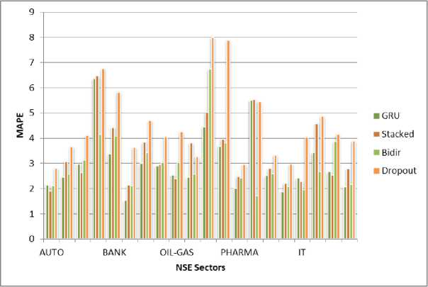
Fig.4. Performance comparison of LSTM variants

Contrary to their initial hypothesis, a clear- cut relationship between LSTM variants and specific sectors within the stock market seemed to be absent. Whether the Banking, IT, Pharma, Oil and Gas, or Automobile sector was scrutinized, consistent results were obtained: GRU (Gated Recurrent Unit) emerged as the top performer across the board. This revelation marked a departure from conventional wisdom and challenged established notions within the realm of stock market analysis. Instead of witnessing tailored performances of LSTM variants in accordance with sector-specific characteristics, a uniform superiority of GRU was encountered by the researchers. The implications of this finding resonated far beyond the confines of academic curiosity. For practitioners navigating the intricate landscape of the stock market and researchers seeking to refine predictive models, a pivotal moment was signaled. A critical reassessment of the conventional wisdom surrounding model selection for time series data, particularly within the context of stock market analysis, was prompted. The unexpected dominance of GRU suggested that its inherent characteristics were uniquely equipped to grapple with the intricacies and nuances inherent in the NSE India stock market. Its ability to capture and adapt to complex patterns seemed to outshine the purported advantages of other LSTM variants. In essence, the importance of comprehensive evaluation and empirical validation was underscored by these results. A reminder was served that while theoretical frameworks and hypotheses provide valuable guidance; empirical evidence often unravels its own narrative, one that may deviate from initial expectations. As this insight is absorbed by practitioners and researchers alike, they are compelled to reconsider their approach to model selection, prioritizing empirical performance over theoretical conjecture.

ensures a comprehensive evaluation of GRU's effectiveness in financial time series forecasting and sets the stage for potential refinements or optimizations to enhance the model's performance in handling complex financial data.

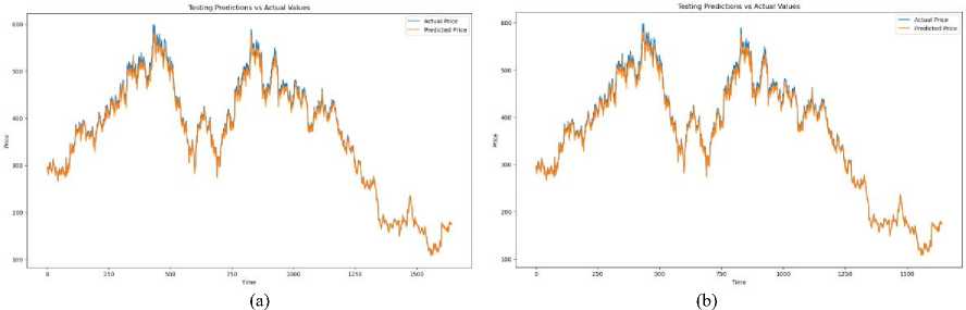
Fig.5. (a) LSTM prediction using complex dataset (b) GRU prediction using complex dataset

Following the trajectory set by the preceding discourse, a meticulous evaluation of both LSTM and GRU models was embarked upon by the experiment, leveraging the dataset of TATA Motors of 20 years from January 2001. The comparative performance of the two models across a large dataset was aimed to be ascertained by this systematic investigation, shedding light on their respective strengths and limitations in the domain of financial time series forecasting. As anticipated, the prowess of GRU was demonstrated by outshining LSTM when tasked with the smaller dataset, mirroring the findings from previous experiments conducted on multiple variants across various sectors of the NSE India. GRU's efficacy in swiftly processing data and extracting meaningful patterns was reaffirmed, thereby showcasing its aptitude for handling moderate- sized datasets common in financial analyses. However, as shown in figure, the plot thickened when the scrutiny extended to encompass the larger dataset spanning two decades. Contrary to expectations, the supremacy of GRU over the base LSTM variants failed to be maintained, faltering in its performance on the expansive and inherently complex dataset. This disparity in performance between the two models underscored certain inherent limitations of the GRU architecture, necessitating a deeper dive into the underlying factors contributing to this discrepancy.

• 4.3.    Assessing Technical Indicators (TIs) to Address Constraints Associated with GRU

GRU, or Gated Recurrent Unit, simplifies the architecture by merging the forget and input gates into a single update gate, and combining the cell state and hidden state into a single vector, thus reducing computational complexity. This streamlined design makes GRU networks computationally less expensive compared to LSTM networks and more efficient in terms of training time and memory usage. However, this simplicity comes at a cost, as the reduced number of gates in GRU may limit its ability to capture complex temporal dependencies and handle long-range dependencies as effectively as LSTM networks.

One of the primary insights gleaned from the experimentation was the struggle of GRU in identifying and leveraging long sequence dependencies embedded within the extensive dataset. Furthermore, light was shed on GRU's susceptibility to noisy data, a common occurrence in lengthy datasets spanning extended timeframes. The inherent noise inherent in long datasets posed a challenge for GRU, potentially exacerbating issues related to vanishing gradient problems and hindering its ability to effectively discern meaningful patterns amidst the noise. In light of these revelations, the discussion pivoted towards addressing the underlying challenges faced by GRU.

To overcome the identified problems of the standard GRU model, a set of carefully selected technical indicators commonly used in financial analysis were introduced. The chosen indicators aimed to provide additional context and features to the model, addressing these challenges.

• A.    Moving Average (MA)

The Moving Average smooths out price data to filter out short-term fluctuations and highlight longer-term trends, which GRU models may not fully capture due to their inherent biases toward recent data. The formula for the simple moving average over a window of n days is:

n - 1

MA = - У P ( t - i )

П i = 0

Where P(t-i) represents the stock price at time t-i. By using this indicator, the model gains insights into long-term price trends, allowing it to balance between recent and older price movements, which help address GRU’s short-term bias.

• B.    Moving Average Convergence Divergence (MACD)

The MACD captures momentum by measuring the difference between a fast and slow exponential moving average (EMA) and provides signals for potential reversals. GRU might struggle to detect sudden trend changes, and MACD helps by providing a leading indicator of momentum. The formula for MACD is:

MACD = EMA_U - EMA₆

Where EMA n represents the exponentially weighted moving average over n days. A signal line, the 9-day EMA of the MACD, is often used to generate buy/sell signals. By incorporating MACD, the model is equipped to recognize changes in momentum, improving its ability to detect turning points, which is essential in capturing trend reversals.

• C.    Relative Strength Index (RSI)

The RSI is a momentum oscillator that measures the speed and change of price movements. GRU models might have difficulty identifying overbought or oversold conditions directly from raw price data. RSI addresses this by normalizing price gains and losses over a window period, typically 14 days. The formula for RSI is:

RSI = 100 -

100 1

1 + RS )

Where RS is the ratio of average gains to average losses over the defined period. This helps the model identify when a stock is potentially overbought or oversold, enhancing its ability to forecast corrections in the market.

• D.    Bollinger Bands

• 4.4.    Results and Insights from Incorporating Technical Indicators into GRU

Bollinger Bands consist of a moving average and two standard deviations (SD) above and below it, which measure volatility. GRU models may underperform in highly volatile environments, and Bollinger Bands provide a volatility measure that allows the model to adjust its predictions in such conditions.

The upper and lower bands are given by:

Upper _ Band = MA + ( K x SD )

Lower _ Band = MA - ( K x SD )

Where k is typically set to 2, and SD is the standard deviation of price over the window. By using Bollinger Bands, the model becomes sensitive to volatility, helping it adapt its predictions based on the dynamic market environment.

A significant stride towards addressing the identified limitations was taken by introducing a novel approach, building upon the insights garnered from the previous phases of experimentation. In order to augment the predictive capabilities of the GRU model, four technical indicators (TIs) were incorporated, enriching the dataset with additional context and features tailored specifically for the intricacies of the stock market dynamics. The rationale behind this modification was based on its potential to empower the models to better discern and leverage long-term dependencies inherent in the financial data. By integrating domain-specific characteristics through the introduction of technical indicators, a more nuanced understanding of the underlying trends and patterns was sought to be provided to the models, thereby enhancing their predictive accuracy and robustness.

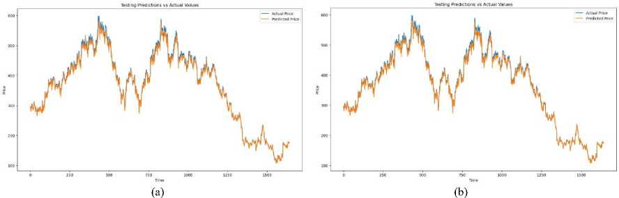
Fig.6. (a) Prediction without integration of TI’s (b) Prediction with integration of TIs

The results yielded from this augmentation were nothing short of remarkable. In a striking revelation, a marked improvement in performance was showcased by the GRU model, bolstered by the inclusion of technical indicators, compared to both its original iteration and the LSTM model. This compelling finding not only underscored the efficacy of the proposed enhancement strategy but also highlighted the adaptability and versatility of the GRU architecture in capturing and leveraging long-term dependencies when furnished with pertinent contextual information.

The augmented GRU model, now enhanced with the selected financial indicators, underwent a huge performance analysis against the traditional LSTM and other variants. The evaluation encompassed many standard metrics. Metrics to identify capabilities in value such as Mean Squared Error (MSE), Mean Absolute Error (MAE), and Root Mean Squared Error (RMSE) were computed to quantify the accuracy of predictions. These standard units were calculated for both short time and longtime prediction horizons.

Table 3. Impact of integration of TIs on Performance of GRU

	Without TIs	With TIs
Train MAE	14.37	13.71
Test MAE	13.97	12.87
Train MAPE	3.09	2.97
Test MAPE	2.85	2.73
Train RMSE	1.29	1.23
Test RMSE	1.22	1.09
Train R2 Score	0.9832	0.9821
Test R2 Score	0.9993	0.9997

Table 3, which serves as a repository of the experimental outcomes, emerged as a crucial artifact encapsulating the essence of the research findings. Through meticulous analysis, the performance disparities between the base LSTM model and the GRU model across datasets of varying magnitudes were delineated by the table. Moreover, a comprehensive overview of the enhancements achieved through the incorporation of technical indicators into the original dataset was provided, shedding light on the transformative impact of domain-specific features on predictive modeling accuracy. By juxtaposing the performance metrics of the base models against the augmented GRU model, Table 3 served as a beacon of insights, illuminating the path towards future advancements in financial time series forecasting methodologies. The findings encapsulated therein not only reaffirmed the superiority of GRU over LSTM in certain contexts but also underscored the untapped potential for further refinement and optimization through the integration of domain-specific knowledge and features. The introduction of technical indicators as a means of enhancing the GRU model represented a pivotal juncture in the research journey, opening new vistas for exploration and innovation in the realm of predictive analytics for financial markets. As researchers continue to unravel the intricacies of time series forecasting, the findings presented in Table 3 are serving as a cornerstone for future endeavors aimed at harnessing the full potential of machine learning models in deciphering the complexities of financial data.

(b)

(a)

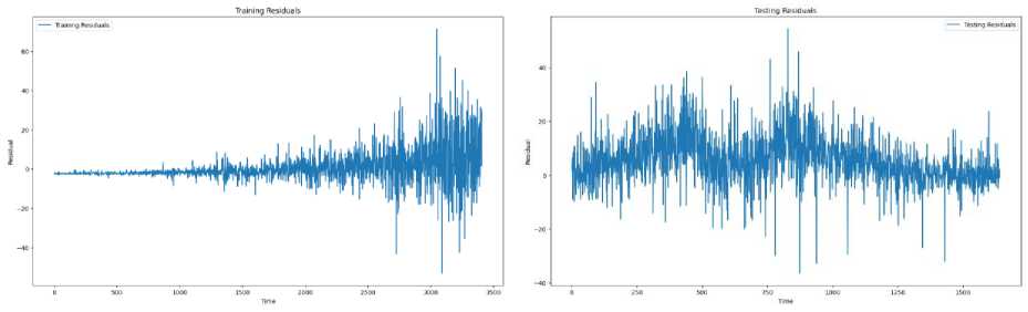
Fig.7. (a) Training residuals (b) Testing residuals

Upon examining the generated residual plot as shown in Fig.7, several key observations can be made. The residuals, which are the differences between the actual and predicted stock prices, appear to be randomly dispersed around the horizontal axis (residual = 0). This suggests that the proposed model does not exhibit systematic bias in its predictions, indicating good predictive performance. Most of the residuals are clustered around the zero line, implying that the majority of the predictions are relatively accurate. However, there are some points where the residuals deviate significantly from zero, indicating occasional larger prediction errors. There is a noticeable pattern in the spread of the residuals over different ranges of predicted values. For instance, larger residuals are observed during periods of high stock price volatility, suggesting heteroscedasticity. This indicates that the prediction accuracy of the proposed model may vary with market conditions, being less accurate during highly volatile periods. No discernible trend or pattern in the residuals were detected, supporting the assumption that the residuals are uncorrelated and the model has captured the underlying stock price movements well. This absence of pattern reinforces the reliability of the proposed model in stock price prediction. An examination of residuals over time shows no significant serial correlation, indicating that residuals are independent of each other. This suggests that the model's errors are not influenced by previous errors, supporting the robustness.

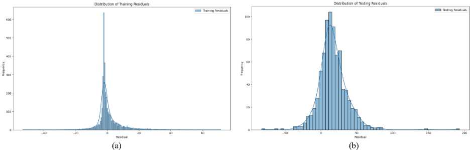
Fig.8. (a) Distribution of training residuals (b) Distribution of testing residuals

As shown in Fig.8, the residuals are symmetrically distributed around zero, indicating that the prediction errors are balanced. This symmetry suggests that the proposed model does not systematically overestimate or underestimate the stock prices. The residuals approximate a normal distribution, with most residuals clustering near zero and fewer residuals found at the extremes. This bell-shaped curve implies that the prediction errors are mostly small, with fewer large errors, aligning with the expected behavior of an effective predictive model. The mean of the residuals is close to zero, further reinforcing the absence of significant bias in the model's predictions. A mean near zero indicates that, on average, the model's predictions are accurate and any errors are equally likely to be positive or negative. The residual distribution exhibits low skewness and kurtosis, suggesting that there are no heavy tails or extreme deviations. This implies that extreme prediction errors are rare, and the residuals do not deviate significantly from the normal distribution. Although the residuals generally follow a normal distribution, a few outliers are present. These outliers represent instances where the model's predictions significantly deviated from the actual stock prices, possibly due to sudden market changes or unique events not captured in the training data. While the residuals are mostly homoscedastic, indicating a consistent variance, there are periods of heteroscedasticity where the spread of residuals increases. This suggests that the prediction accuracy of the proposed model may vary under different market conditions, particularly during high volatility.

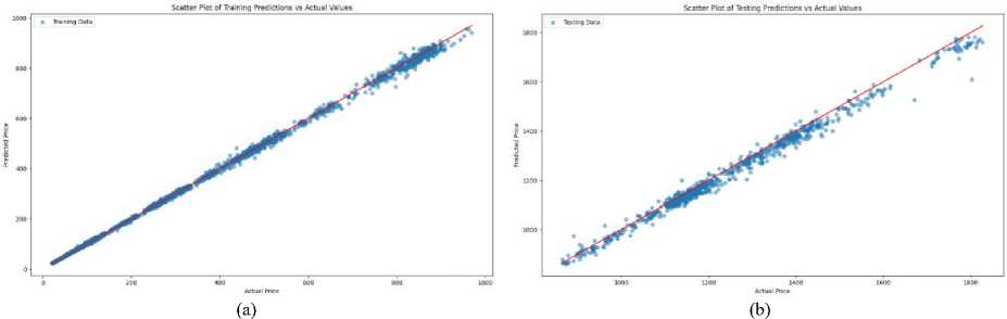
Fig.9. (a) Scatter plot of training predictions vs actual values (b) Scatter plot of testing predictions vs actual values

The scatter plot can be seen in Fig.9. It shows a strong linear relationship between the predicted and actual stock prices, with most points aligning closely along the diagonal line (45-degree line). This alignment indicates that the model’s predictions are generally accurate and proportional to the actual values. A significant clustering of points around the diagonal suggests that the model's predictions closely match the actual stock prices for a majority of the data points. This clustering is a positive indicator of the model's reliability and precision. While most points are near the diagonal, some deviations are present. These deviations indicate instances where the model's predictions were either higher or lower than the actual stock prices, highlighting areas where the model could be refined for better accuracy. The scatter plot covers a wide range of stock prices, demonstrating the model's ability to handle different stock price levels. However, there may be a slight widening of the spread of points at higher stock prices, indicating that prediction accuracy may decrease as stock prices increase. The density of points is higher around moderate stock price levels and lower at extreme high or low prices. This pattern suggests that the model is more frequently predicting within a central range, possibly reflecting the distribution of the training data.

(a)

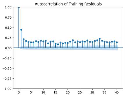
Fig.10. (a) Autocorrelation and training residuals (b) Autocorrelation and testing residuals

The error autocorrelation plot as shown in Fig.10 shows minimal autocorrelation at different lags, indicating that prediction errors are not significantly correlated with previous errors. This suggests that the model's errors are independent and not influenced by past prediction errors, which is a positive sign of model robustness. The autocorrelation values hover close to zero across various lags, demonstrating that the prediction errors are randomly distributed. This randomness implies that the model does not exhibit any temporal patterns or systematic errors, reinforcing the model's effectiveness in handling time series data. There are occasional spikes in the autocorrelation plot, which may indicate outliers or periods where prediction errors show some level of correlation. These spikes suggest that there could be specific times or conditions where the model's performance is less reliable, potentially due to sudden market events or structural changes. The plot's confidence intervals are generally within the range of the autocorrelation values, indicating that the observed autocorrelation is not statistically significant. This supports the notion that the model's errors do not exhibit strong dependencies over time. The absence of a clear pattern in the autocorrelation plot suggests that the model's errors are not systematically influenced by past errors. This lack of pattern reinforces the reliability of the proposed method in producing independent and uncorrelated prediction errors. The plot reveals some variability in autocorrelation values, which may point to varying levels of prediction accuracy over different time periods. This variability could indicate that the model's performance is influenced by changing market conditions or other external factors.

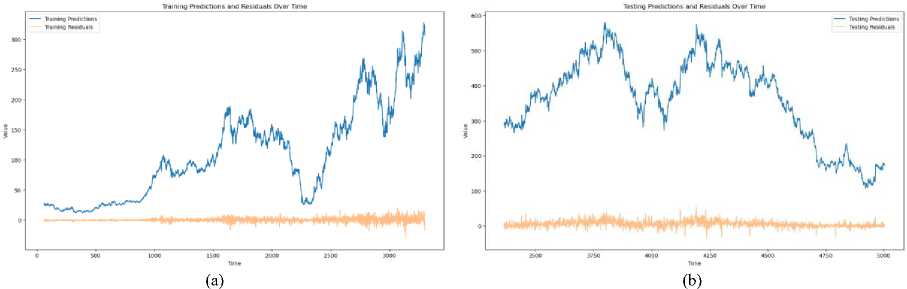
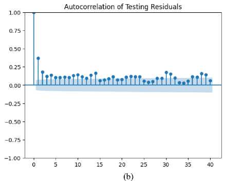
Fig.11. (a) Training predictions and residuals over Time (b) Testing predictions and residuals over time

The plot of predictions over time shows a generally consistent trend with the actual stock prices, reflecting the model's ability to capture the underlying movement of the stock. This consistency suggests that the proposed method effectively tracks the overall direction and magnitude of stock price changes. Fig.11 shows that the residuals, which are the differences between the predicted and actual values, exhibit variability over time. While residuals are relatively small during stable periods, they tend to increase during periods of high volatility or market turbulence. This pattern indicates that the model's accuracy may decrease during turbulent market conditions. The residual plot reveals no significant long-term trend, suggesting that the proposed method does not exhibit systematic drift or bias over time. Residuals appear to fluctuate around zero, which is indicative of the model's stability and its capacity to adapt to different market conditions without introducing persistent errors. Certain spikes or clusters in the residuals correspond to major market events or anomalies. These spikes highlight instances where the model's predictions deviated substantially from actual values, possibly due to unforeseen market shocks or structural changes not captured by the model. There is noticeable variability in the magnitude of residuals across different time periods. Larger residuals are observed during high-volatility periods, indicating that the model's performance may vary with market dynamics. This variability suggests that while the model performs well under normal conditions, it may need adjustments to handle extreme market fluctuations more effectively. The residuals do not show a strong correlation with the predictions themselves, which indicates that, the prediction errors are not systematically related to the magnitude of the predicted values. This lack of correlation supports the idea that the model's errors are random and not influenced by the size of the predictions.

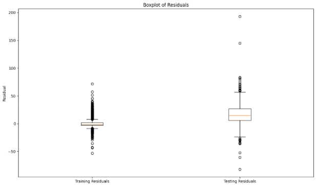
Fig.12. Boxplot of residuals

The median of the residuals is close to zero, indicating that the average prediction error is minimal. This suggests that the proposed method does not have a systematic bias in its predictions, as the median residual being near zero reflects balanced overestimation and underestimation. The interquartile ranges (IQR), represented by the box in the boxplot, and shows the central 50% of residuals. We can see this in Fig.12. A relatively narrow IQR implies that the majority of residuals are tightly grouped around the median, indicating consistent prediction accuracy for most of the data. Conversely, a wide IQR would suggest greater variability in prediction errors. The boxplot reveals a number of residuals outside the "whiskers," which represent potential outliers. These outliers are points where the prediction errors are significantly higher or lower than the typical range of residuals. The presence of outliers indicates that the model occasionally produces predictions with substantial errors, possibly due to extreme market conditions or anomalies. The whiskers extending from the box represent the range of residuals within 1.5 times the IQR from the quartiles. Residuals beyond this range are considered outliers. If the whiskers are relatively short, it suggests that the residuals do not deviate far from the central range. Long whiskers would indicate a wider spread of residuals. The boxplot's symmetry can provide insights into the skewness of the residuals. If the box and whiskers are not symmetrical around the median, it suggests skewness in the residuals. For example, a longer whisker on one side may indicate a tendency for larger positive or negative errors. The shape of the box and the length of the whiskers can give insights into the overall distribution of residuals. A box that is skewed or has asymmetrical whiskers indicates that the residuals might be influenced by specific patterns or external factors not fully captured by the model.

• 4.5.    Discussion

5.    Conclusions and Future Works

The superior performance of the Gated Recurrent Unit (GRU) over the Long Short-Term Memory (LSTM) model in the absence of technical indicators was unexpectedly revealed, serving as a catalyst for the reevaluation of preconceived notions and assumptions. This unforeseen outcome challenged the conventional wisdom surrounding the comparative efficacy of these two recurrent neural network architectures in the domain of financial time series forecasting. However, the subsequent success of GRU, particularly when augmented with technical indicators, ushered in a paradigmatic shift in our understanding of model behavior and the efficacy of feature engineering in addressing inherent limitations. The transformative potential of feature engineering in mitigating the limitations of recurrent neural networks was underscored by the study's findings, paving the way for enhanced predictive capabilities in financial time series forecasting. The superiority of GRU, especially when supplemented with domain-specific features, emphasized the pivotal role of contextual information in bolstering the models' capacity to discern and leverage long-term dependencies embedded within stock market data. This nuanced understanding of model behavior underscores the need for a tailored approach to model selection, wherein the choice between LSTM and GRU hinges upon the availability and incorporation of relevant domain-specific features. Moreover, the practical implications of these findings were highlighted by the study, elucidating the critical importance of feature selection methods in maximizing the predictive efficacy of recurrent neural networks for time series data. By emphasizing the effectiveness of feature engineering in enhancing model performance, actionable insights with tangible real-world applications, particularly in the volatile and intricate domain of stock markets, were offered by the research, transcending theoretical frameworks. Moving forward, further research endeavors aimed at optimizing technical indicator selection and hyperparameter tuning to refine the proposed model were advocated by the study. This iterative approach to model refinement underscores the dynamic nature of research in machine learning and underscores the need for continuous innovation and exploration in pursuit of enhanced predictive capabilities. In conclusion, a significant milestone in the realm of financial time series forecasting was represented by the study's findings, shedding light on the untapped potential of GRU and the transformative power of feature engineering in addressing inherent limitations. By transcending traditional paradigms and advocating for a nuanced understanding of model behavior, a roadmap for maximizing the predictive efficacy of recurrent neural networks in unraveling the complexities of financial markets was offered by the research.

In conclusion, insightful findings challenging prevailing assumptions have been yielded by our investigation into time series prediction in the NSE India stock market. Contrary to expectations, consistent outperformance across various sectors by Gated Recurrent Unit (GRU) variants over other variants of Long and Short Term Memory (LSTM) has been observed, highlighting the need for a reassessment of model preferences in the context of stock exchange prediction. The dynamic nature of the financial markets is underscored by this unexpected outcome, where the advantageous inherent characteristics of GRU for capturing complex patterns and behaviors are emphasized.

While GRU emerges as the superior choice over LSTM for small datasets due to its efficiency, it faces challenges with larger datasets characterized by greater complexity and long dependencies. The identified limitations have been addressed by integrating suitable technical indicators holds promise for overcoming these hurdles and significantly enhancing GRU's performance in such scenarios. Future research efforts should focus on refining these approaches to maximize the effectiveness of GRU models in handling large and intricate datasets. One promising direction is to explore the integration of advanced feature selection methods such as Principal Component Analysis (PCA) or Recursive Feature Elimination (RFE). Use of F-regression, Mutual information may greatly enhance performance. This would allow for a more refined input selection, which may lead to better generalization and performance, especially in volatile market conditions. Additionally, hybridizing GRU with other deep learning architectures, such as NBEATS, attention mechanisms or transformers, could further improve the model's ability to capture long-term dependencies and trends in stock data.

The proposed approach could be extended to other financial markets to assess its generalizability. Additionally, further investigations could focus on optimizing hyper parameters, exploring additional technical indicators, and finetuning the model architecture to improve interpretability and transparency. This study will be highly beneficial for investors, traders, and financial analysts by providing accurate stock price predictions that support decision-making in portfolio management, algorithmic trading strategies, financial risk assessment and market sentiment analysis