Comparative descriptive analysis of breast cancer tissues using k-means and self-organizing map

Published Online August 2018 in MECS

In computational science, principles, techniques, and theories within and outside the discipline especially biologically inspired ones are applied to real life problems. At its classic, hard computational theories are applied to diverse domains to solve problems that range from the simple mathematical to more complex engineering and business tasks. However, some problems demand for cognitive solutions and these are handled by intelligent systems that have human-like intelligence planted in them. One of the applications of these intelligent computational theories is Artificial Intelligence in Medicine (AIM) where computational ideas from conventional AI and or computational intelligence are employed in delivering an improved healthcare. In conventional AI, machine learning algorithms are sometimes used to detect meaningful relationships in a clinical dataset so as to diagnose, treat, and predict possible outcomes. Although the final predictions or diagnosis of intelligent systems are not always accepted as final but they are mostly accepted as aiding tools in decision making as they tend more to provide decision support than final decision especially in deadly diseases’ diagnosis.

Among these deadly diseases is Cancer. It is caused by abnormal cell growth and which spreads to other parts of the body. Among different types of cancer, breast cancer is the most prevalent and serious public health problem amidst women in the world [1]. Breast cancer usually occurs in the fibro glandular area of breast tissue [2] and which when early detected can be easily cured. Mammography is one of the imaging tests used for early detection of cancerous cells in the breast tissues. Others include Breast Ultrasound, Breast Magnetic Resonance Imaging (MRI) and newer experimental imaging tests among which is the Electrical Impedance Imaging (EII) that scans the breast for electrical conductivity with a strong idea that cancerous cells conducts electricity differently from normal cells. The EII test passes a minute electrical current through the breast and then detects it using small electrodes tapped to the breast’s skin. The results of the tests generate voluminous dataset that need been analyzed by radiologists or other appropriate medical personnel. However, variations in radiologists’ interpretations especially mammograms [3,4] due to the fact that the task is repetitive and timeconsuming has been a problem. The need for interpretation reproducibility which will bring about a reliable result and subsequent early detection, treatment and mortality’s rate reduction has been the concerns of computational scientists as they have been providing computer aided tools in automating the process of scans’ interpretation and other statistical results of cancer screening.

In this paper, dataset with electrical impedance measurements in samples of freshly excised tissues from the breasts of some volunteers are clustered using K-means, X-means-improved K-means and Self-Organizing Map all implemented using R i368 version 3.4.2 for the purpose of identifying the best clustering method out of the three. The dataset [5], by [6,7] had impedance measurements made at the frequencies: 15.625, 31.25, 62.5, 125, 250, 500, 1000 KHz. The attributes of the dataset include Impedivity (ohm) at zero frequency (IO), phase angle at 500 KHz, high-frequency slope of phase angle, impedance distance (DA) between spectral ends, area under spectrum, area normalized by DA, maximum of the spectrum, distance between IO and real part of the maximum frequency point, and length of the spectral curve. The paper is organized as; section two, discussing related work while methods and materials used in the study appear in section three. Experimental setup, results and discussions are contained in sections four and five respectively while section six provides conclusive points and recommendations for upcoming researchers who may which improving on the study.

• II.    R elated W ork

  Several studies have been carried out on the detection and classification of breast cancer especially from mammograms. Chan et al., (1995) classified breast tissue on mammograms into masses and normal. In the study, they used texture features derived from spatial grey level dependency (SGLD) matrix and stepwise linear discriminant analysis to perform the 2-class classification. The classifier could achieve an average area (Az= 0.84 during training and Az=0.82 during testing) under the receiver operating characteristics (ROC) curve [8].

Wang and Karayiannis (1998) presented another approach to detecting micro-calcifications in digital mammograms using wavelet-based sub-band image decomposition, and then reconstructing the mammogram (that contains only high-frequency components, including the micro-calcifications) from the sub-bands containing only high frequencies [9].

Garma et al., (2014) proposed a method for detection of breast cancer based on digital mammogram analysis. Haralick texture features were derived from SGLD matrix. The features were extracted from each region of interest (ROIs). The features discriminating to detect abnormal from normal tissues were determined by stepwise linear discriminant analysis classifier. The proposed method achieved 95.7% of relative accuracy for classification of breast tissues based on digital mammogram texture analysis [10].

Sheshadri and Kandaswamy in a study used statistics extracted from mammograms to classify breast tissue. The statistical features extracted are the mean, standard deviation, smoothness, third moment, uniformity and entropy which signify the important texture features of breast tissue were used to obtain four basic classes of breast tissues (fatty, uncompressed fatty, dense and high density). The method was evaluated with the data given in the data base (mini-MIAS database) and obtained accuracy of 78% [11].

Leonardo et al., (2006) in a work analyzes the application of the co-occurrence matrix to the characterization of breast tissue as normal, benign or malignant in mammograms. The characterization is based on a process that selects using forward selection technique from all computed measures which best discriminate among normal, benign and malignant tissues. A Bayesian neural network is used to evaluate the ability of these features to predict the classification for each tissue sample. The proposed method was evaluated using a set of 218 tissues samples, 68 benign and 51 malignant and 99 normal tissues. The result of the evaluation provided an accuracy of 86.84% [4].

Zhang et al., (2005) in their work to breast tissue classification from mammograms, applied a neural-genetic algorithm for feature selection in conjunction with neural and statistical classifiers has obtained a classification rate of 85.0% for a test set [13].

Christoyianni et al., (2002) proposed a special neural network in which a Radial Basis Function Neural Network (RBFNN) is used in the classification of breast tissues from mammograms. The network was evaluated using data from the MIAS Database with a recognition accuracy of 88.23% in the detection of all kinds of abnormalities and 79.31% in the task of distinguishing between benign and malignant regions [14].

Nithya and Santhi (2017) presented a computer-aided diagnosis (CAD) system for breast density classification in digital mammographic images. The proposed method consists of four steps: (i) breast region is segmented from the mammogram images by removing the background and pectoral muscle (ii) segmentation of fatty and dense tissue (iii) percentage of the fatty and dense tissue area is calculated (iv) Classification of breast density. Results of the proposed method evaluated on the Mammographic Image Analysis Society (MIAS) database. The experimental results show that the proposed CAD system can well characterize the breast tissue types in mammogram images [15].

Petroudi et al., (2003) presented a new approach to breast tissue classification using parenchymal pattern where they developed an automatic breast region segmentation algorithm that accurately identifies the breast edge, as well as removing the pectoral muscle in Medio-Lateral Oblique (MLO) mammograms. The approach uses texture models to capture the mammographic appearance within the breast area: parenchymal density patterns are modeled as a statistical distribution of clustered, rotationally invariant filter responses in a low dimensional space. This robust representation accommodates large variations in intraclass mammogram appearance and can be trained in a straight-forward manner.

• III.    R esearch M ethodology

This section discusses the methodology of the study and it involves both hardware and software materials and techniques used for the designs, implementations and evaluations of the proposed algorithms. These are discussed shortly:

• A.    Materials

With the hardware materials used, little attention is given to it in this study as the researchers believe that any personal computer with hardware configuration that supports R i368 version 3.4.2 and windows 7 Ultimate or newer versions would be appropriate for implementing the algorithms as this was considered during the course of the study. The software tools used include R i368 version 3.4.2, a data analytical package for data analysis and knowledge discovery and Weka version 3.6.3 (Waikato Environment for Knowledge Analysis) used for optimizing attributes selected for the analysis. The former was used for implementing K-means and SOM which were the algorithms used during the course of executing this study.

The dataset analyzed here was taken from a study [6,7] of 106 freshly excised breast tissue samples performed in the range of 15.625Hz to 1MHz and this data is available publicly at the UCI Machine Learning Repository. Histological analysis was performed to classify each tissue sample as carcinoma (car), fibro-adenoma (fad), mastopathy (mas), glandular (gla), connective (con), or adipose (adi) tissue. The dataset has 9 attributes, IO: Impedance (ohm) at 0Hz; PA500: Phase angle at 500 kHz; HFS: High-frequency slope of the phase angle; DA: Distance between ends of the impedance spectrum; AREA: Area under the impedance spectrum; A/DA: AREA normalized by DA; MAX IP: Maximum of the spectrum; DR: Distance between I0 and the real component of the maximum frequency point; and P: Length of the spectral curve.

• B.    Methods

This section discusses methods used for data preprocessing, clustering and evaluation.

• i.    K-means Algorithm

n

E( x- y i)

i =1

Step 1: Select K data po nts as n t al centro ds

Step 2: Repeat

• a.    Form K clusters by ass gn ng each po nt to ts closest centro d us ng d stance norm (1)

• b.    Re-compute centro d of each cluster by comput ng we ghted means of all ts po nts us ng:

  X =

  
  

  E ” = t ⁽ y * w )

  E >

  
  
  
  

where, y =data po nt and w =we ght of data po nt y

Step 3: Unt l centro ds do not change

n

SSE = _EE dst ( C , x ) 2 i =1 X6C_i

where,

SSE is the sum of squared errors (the objective function for K-Means), and;

dist(c i , x) ² = Euclidean distance measure between input x and ith centroid (i.e. c i ).

The goal of K-means is to minimize the objective error function in (3)

• ii.    K Selection and K-centroids Initialization

It is believed that the result of K-means is greatly influenced by “k” clusters specified by the analyst and also the initial centroids chosen. In this study, elbow method that finds the optimal number of clusters for a dataset by incrementally varying the cluster number “k” starting from 2 and determining the computational cost (usually sum of squared errors) of the clustering as “k” increases. A value is reached that is called the elbow value where the computational cost reduces sharply and from which subsequent decrease seems insignificant (Fig. 1). Also, a hierarchical clustering of the dataset is taken to predetermine the number of likely clusters that exists in the dataset (Fig. 2).

From Fig. 1, the noticeable elbow value is 4, but with the pattern as contained in the dataset, there are six clusters available in the dataset. Therefore, in this study, both 4 and 6 are considered as possible clusters for the dataset and used in the clustering. Other method for “k” determination is information criterion approach (Akaike criterion or Bayesian criterion) but, elbow method and plot of hierarchical clustering are considered in this paper.

Random selection of initial centroids for multiple running of the algorithm is considered in this paper. The centroids are samples from the dataset.

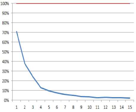
Fig.1. chart showing elbow values as possible values of clusters from the dataset

• iii.    SOM

Self-organizing map is self-features organizing algorithm that learns without the aid of human intervention. It operates on the basis of neighborhood function to cluster data points into their groups. Its operation is stated as:

For each input object xs in the dataset perform the following four steps:

Step 1: Find the neuron with the most 'distinguished' response of all using Euclidean distance norm

Step 2: The maximal neighborhood around this central neuron is determined (usually two rings of neurons around the central neuron)

Step3: The correction factor is calculated for each neighborhood ring separately

Step 4: The weights in neurons of each neighborhood are corrected according to (4)

wt (new) = wt (old) + n(t)a(d(c - j), t)(xSJ - w (old))

where, x _s =input

(t)=learning rate usually selected randomly between 0

and 1 (but, in this paper, t ranges from 0.05 to 0.01) a(.)=neighborhood function and it depends on two parameters:

• •    One is the topological distance d(c-j) of the j-th neuron from the central one and

• •    The second parameter is time of training (t)

SOM operates is a similar manner to K-means that is, it groups data points into clusters. However, it additional maintains the neighborhood arrangements of the data groups as similar groups lie close to one another on the map.

• IV.    E xperimental P ilot

This section considers experimental pilot on the implementation of the machine learning algorithms in R i368 version 3.4.2 and their evaluations with breast tissue dataset.

• A.    Data Preprocessing

Prior to the use of the R, optimized selection of attributes out of the dataset’s nine attributes was considered using various search algorithms implemented in WEKA 3.6.3. The dataset has 106 instances and 9 attributes before preprocessing. During the preprocessing, data with instance number 103 was removed as it posed as an outlier therefore having 105 instances of data left for the analysis. Out of the nine attributes, Genetic, Greedy stepwise, Best First and Exhaustive Search techniques were used for the selection of the best optimized attributes that could be used for the analysis. IO, HFS, A/DA and Max IP are optimized attributes for Genetic, Greedy stepwise, and Exhaustive Search techniques while IO, A/DA and Max IP are the optimized attributes for Best First Search technique. The dataset was normalized using min-max technique modeled as (5) and finally scaled using scale () function in R.

v ^{, (} i ) =

(v (i)- min [ v (i)])

(max [ v (i)]- min [ v (i)])

where, v(i) is the original value and v ^, (i) is the normalized value

Cluster Dendrogram

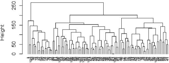
Fig.2. Hierarchical clustering of the dataset to predetermine the number of likely clusters using R

dist(breast) hclust (*, "complete")

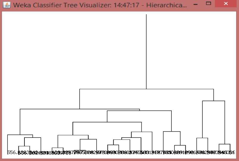
Fig.3. Hierarchical clustering of the dataset to predetermine the number of likely clusters using WEKA

• B.    Experimental Pilot with K-means

This part of the study considers implementation of K-Means algorithm in R and execution of it with the preprocessed dataset.

Case 1: Using IO, A/DA and Max IP as Best First search selected attributes:

K-means algorithm was implemented in R and used on 105 instances of the dataset. The algorithm used 20 samples of randomly selected initial centroids and in each initialization, it runs for 100 times. The best result for the 20 running is chosen as the final output as contained in Fig. 4 and Fig. 5. In Fig. 4, fours clusters were considered while in Fig. 5, six clusters were considered.

Case 2: Using IO, HFS, A/DA and Max IP as Exhaustive, Greedy Stepwise, and Genetic Search selected attributes:

The implemented K-means algorithm considered 20 samples of randomly selected initial centroids and in each initialization, it runs for 100 iterations. The best result for the 20 running is chosen as the final output as contained in Fig. 6 and Fig. 7 having dataset grouped into four and six clusters respectively.

• C.    Experimental Pilot with SOM

1 1.1372905 -0.01267169 0.44535190 2 1.2133025 2.13724245 2.26327332

Using IO, A/DA and Max IP as Best First search selected attributes:

In R, package “kohonen” has three functions for selforganizing mapping of input space with output space. These include som, xyf, and supersom. However, the classic function “som” was used for the mapping of the high-dimensional inputs space to low-dimensional outputs space. The maps consist of six and four neurons that are hexagonally arranged to yield six and four clusters respectively. The maps have running lengths of 700 and other attributes were set to their default values in R. 105 scaled instances of the dataset were fed as inputs to the map. Where IO, A/DA and Max IP attributes were the optimized attributes used to represent the nine attributes of the original dataset. The training progress for the 2X3 SOM is shown in Fig. 8 while Fig. 9 shows that of the 2X2 SOM.

Cluster means:

10        A. DA HaxIF

2 -0.6464331 -0.67267170 -0.60503368

3 -0.5013625 0.59025557 -0.03290691

Clustering vector:

[1] 3333332233333333333332222222222222222

[35] 2222222222222323222222222222222221112

[75] 1222111111114141444111144444114

Within cluster suit of squares by cluster:

• [ 1] 14.923542 7.654344 5.069504 27.016865

(between_55 / total_SS = 82.5 %)Available components:

• [ 1] "cluster^-      "centers^-      "tatss"        "withinss" "tot.withinss"

[б|] "betweenss"    "size-          "iter"          "ifault"

Fig.4. Centroids of the Four Clusters of the Dataset

X-ir.eans clustering with	6 clusters	□ f	sizes	52,	10,	zz ,	5,	2 f	14
Cluster means:
10        A.DA	MaxIF
1 -0.6464617 -0.6555357	-0.6067034
2  1.6157226  0.9244350	1.2531454
3 -0.5059213  0.5615535	-0.1022416
4  2.2129046  2.1565020	3.3396324
5  1.4712420  3.5633094	1.2106331
6 1.0441461 -0.2365213	0.1354993
Clustering vector:
[1] 333333113	3 3 3 3 3 3	3	3 3 3	3 3	2 2	2 2	2	1 1	222222222
[33] 222222222	11113 1	3	3 2 2	2 2	2 2	2 2	2	1 1	222226262
[75] 622266 6 66	6 2 6 4 6 5	6	2 4 2	z z	2 6	4 4	4	2 5	6 2 2
Within cluster suit. of senates bv clust
[1] 6.993457 5.664345 5.	.374992 5.05412		2 1.59	13115	: 3.	51245
(betweenSS / total_55	=  91.0%)

Available components

[1] "cluster"      "centers" [6] "betweenss-    "size"

"totss1'1         "withinss"     "tot .withinss" "iter"         "ifault"

Fig.5. Centroids of the Six Clusters of the Dataset

10        HF5       A.DA      MaxIF

• 1  1.3469343 -0.49409-34  0.2569434  0.5994951

• 2    -0.6040005  1.3275269  0.2003353 -0.2105150

• 3  1.Э262ЭОЭ  1.1250796  2.3345060  2.6660033

• 4    -0.5633727 -0.4-518661 -0.5216276 -0.5363027

Clustering vector:

[1] 4242244222244222422224444444444444442

[33] 2444244444444242444244444444444421144

• [7 5] '_ ^ ^ ^ '_'_'_ ^ '_•_•_•_ l '_ l l l              l l l '_ l '_'_ '_

  Within cluster sure, of squares by cluster: [1] 29.52969 24.30639 27.01010 32.54236 (between_55 / total_55 =  "2.6 %)

• [ 1] "cluster"      "centers"      "totss"        "withinss" "tot.withinss"

• ( 6] "betweenss"    "size"         "iter"         "ifault"

Fig.6. Centroids of the Four Clusters of the Dataset

I 0          HF5         A.DA       HaxIF

• 1    -0.63-36697  0.6---6244 -0.39366994 -0.39677035

• 2    -0.6255655 -0.55665642 -0.62145534 -0.60373129

• 3  2.2129046  1.65342524  2.1-3650202  3.3-396-3242

• 4  0.7Э51422 -0.74012554 -0.03-369--- 0.12670170

• 5    -0.5437417  1.77220195  0.66362932 -0.0-350570-3

• 6   1.5941425 -0.02467592  1.36424740  1.24606251

• [1]    2545522155544515215512222222222212221

[33] 1122122221222115222122222222222214642

• [75]    4 2 1 2 4 4 4 4 4 4 6 4 34646366664 33366466

• [1]  7.366931 14.161539  7.742773 15.-37302 9  3.595956 24.307660

(between_SS / total_5S = Sl.O %)

Available components:

• [1]    "cluster"      "centers"      "totss"        "withinss" "tot.withinss"

• [6]    "betweenss""size""iter""ifault"

Fig.7. Centroids of the Six Clusters of the Dataset

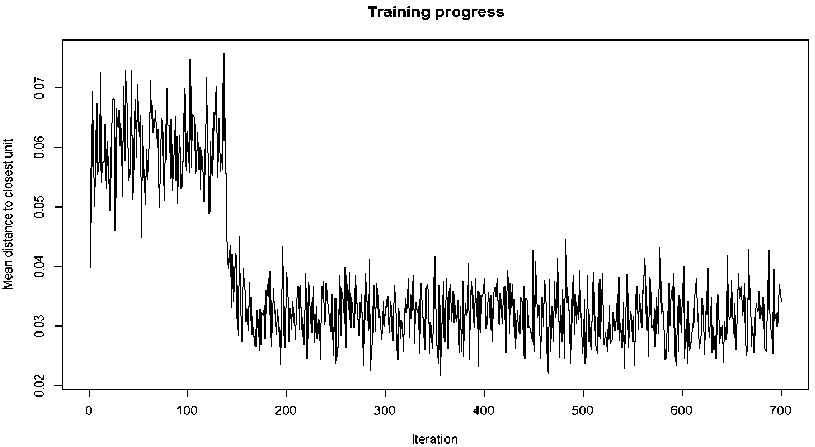
Fig.8. Training progress for SOM with six clusters

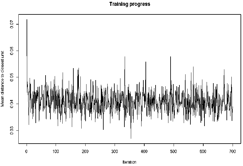
Fig.9. Training progress for SOM with four clusters

D. Discussion

The results of the experimental pilots using K-means and self-organizing map are discussed in this section of the paper. The k-means clustering of the dataset into four and six clusters as presented in Fig. 4 and 5 respectively have confusion matrices (table 1 and table 2); while Fig. 6 and Fig. 7 have their respective confusion matrices as table 3 and table 4.

Table 1. confusion matrix for k-means clustering of dataset into four clusters for case 1

Cluster	1	2	3	4
adi	0	0	10	11
car	19	2	0	0
con	0	4	10	0
fad	0	15	0	0
gla	0	16	0	0
Mas	2	16	0	0

Table 2. confusion matrix for k-means clustering of dataset into six clusters for case 1

Cluster	1	2	3	4	5	6
adi	0	9	5	0	2	5
car	2	0	0	19	0	0
con	4	0	1	0	0	9
fad	15	0	0	0	0	0
gla	16	0	0	0	0	0
mas	15	0	0	3	0	0

Table 3. confusion matrix for k-means clustering of dataset into four clusters for case 2

Cluster	1	2	3	4
adi	13	0	8	0
car	0	14	0	7
con	8	0	0	6
fad	0	0	0	15
gla	0	2	0	14
mas	0	5	0	13

Table 4. confusion matrix for k-means clustering of dataset into six clusters for case 2

Cluster	1	2	3	4	5	6
adi	0	0	5	5	0	11
car	4	4	0	3	10	0
con	1	3	0	9	0	1
fad	1	14	0	0	0	0
gla	2	14	0	0	0	0
mas	7	10	0	0	1	0

Table 6. confusion matrix for SOM clustering of dataset into six clusters for case 1

Cluster	1	2	3	4	5	6
adi	0	9	5	0	5	2
car	19	0	0	2	0	0
con	0	1	0	4	9	0
fad	0	0	0	15	0	0
gla	0	0	0	16	0	0
mass	3	0	0	15	0	0

Table 7. confusion matrix for SOM clustering of dataset into four clusters for case 2

Cluster	1	2	3	4
Adi	0	0	11	10
Car	0	19	0	2
Con	10	0	0	4
Fad	0	0	0	15
Gla	0	0	0	16
Mass	0	3	0	15

Table 8. confusion matrix for SOM clustering of dataset into six clusters for case 2

Cluster	1	2	3	4	5	6
adi	0	9	5	0	5	2
car	19	0	0	2	0	0
con	0	1	0	4	9	0
fad	0	0	0	15	0	0
gla	0	0	0	16	0	0
mass	3	0	0	15	0	0

As illustrated in Fig. 1 and Fig. 2, the natural clusters of the dataset is four. This is supported by the confusion matrix as contained on table 2 as cluster “3” and cluster “5” contain data instances that were wrongly grouped. Also, for case 2 on K-means, table 4 shows cluster “1” and cluster “3” containing data instances that were wrongly grouped. SOMs clustering for case 1 have their performances evaluated with confusion matrices table 5 and table 6 for 2X2 and 2X3 maps while SOMs clustering for case 2 have their performances evaluated with confusion matrices table 5 and table 6 for 2X2 and 2X3 maps.

Table 5. confusion matrix for SOM clustering of dataset into four clusters for case 1

Cluster	1	2	3	4
adi	10	0	11	0
car	0	19	0	2
con	10	0	0	4
fad	0	0	0	15
gla	0	0	0	16
mass	0	3	0	15

For case 1, the K-means with 4 clusters slightly outperforms the SOM with 4 clusters as it misclassified 2 mastopathy breast tissues while the 2X2 SOM misclassified 3 with other classifications been the same. Also, for case 2, it is still observed that K-means performed slightly better than the SOM in classification’s precision.

• V. C onclusion

The process of clinical decision making involves analysing often voluminous medical dataset (which are often erroneous when done by men as there are always introduction of human error into the analysis) to infer knowledge that are made. However, when the analysis is being automated then human error is avoided and an improved result comes in, to aid better clinical decisions. In this study, two machine learning algorithms that carry out self-learning were experimented on dataset (the dataset that is publicly available in the UCI Machine Learning Repository) with electrical impedance measurements in samples of freshly excised tissues from the breasts of some volunteers. Results of the experiment as presented in the paper shows that K-means algorithm to slightly outperforms the self-organizing map in its accuracy. Further researches on comparative analysis of the two algorithms are advised to be experimented with datasets that have more instances and attributes. Also, other variants of the k-means and SOM should be combined and evaluated to provide a better generalization on the best among them when it comes to unsupervised clustering.

A cknowledgements

We acknowledge the supports of all fellows who have in one form or the other contributed to the success of this paper especially, Professor O. Olabode of the Department of Computer Sciences, Federal University of Technology, Akure, Nigeria and all members of staff and students of Departments of Computer Science, Federal University of Technology, Akure, and Mathematical Sciences, Kings University, Odeomu, Nigeria.