Comparative Study between ARX and ARMAX System Identification

Published Online February 2017 in MECS

Intelligent Systems and Robotics Lab, Iranian Institute of Advanced Science and Technology (IRAN SSP), Shiraz/Iran E-mail: ,

• I.    System’S Data Collection

It is a well known fact that real physical systems (engineering systems) are very often uncertain or vague, which generally makes it difficult to accurately model a complex system or process by a mathematical model. Uncertainty means the exact output of a real physical system cannot be predicted by a mathematical model that describes the physical system under investigation, even if the input to the system is known. Uncertainty arises from two sources: unknown or unpredictable inputs (e.g., disturbance, noise) and unknown or unpredictable dynamics. Dynamic models are used for many purposes, to explain system behavior, for control design (i.e., model-based control) and for simulation. As a particular field of application, in motion control of robot manipulators, a dynamic model determines the control inputs needed to realize a reference motion and it also enables an analysis of how particular dynamic effects influence overall robot manipulator behavior. It is therefore important to model system dynamics. Since the model of a system dynamics can at best be an approximation of real physical systems, it will only capture some properties of real system.

Motors are very important instruments in any industries. The applications of motors are wide such as,

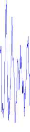
Fig.2. Behavior of Step Function system input-output Modeling

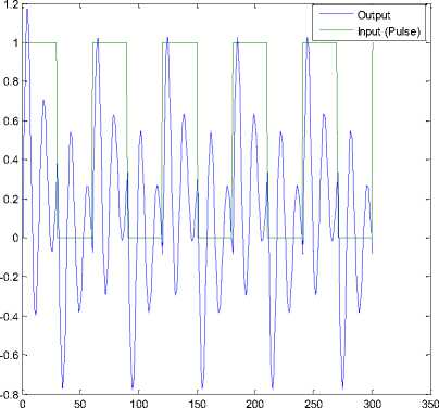
Fig.3. Behavior of Pulse Function system input-output Modeling

Fig.4. Behavior of Triangular Function system input-output Modeling

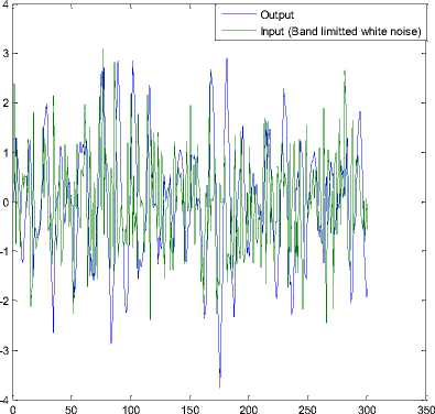
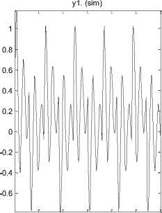
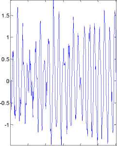
Fig.5. Behavior of Band limited white noise Function system inputoutput Modeling

Figure 2 shows the behavior of input-output data modeling in step input.

Figure 3 shows the pulse input-output behavior system modeling.

Figure 4 shows the triangular input-output behavior system modeling.

Finally in Figure 6, the input random number inputoutput behavior system is modeling.

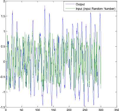
Fig.6. Behavior of input random number Function system input-output Modeling

• II.    Arx System’S Identification

The system modeling and identification is divided into two main groups:

• 1.  Traditional system identification

• 2.  Intelligent system identification.

The classical logical methods of modeling, reasoning, and computing are deterministic. A statement can be true or false and nothing in between, or a variable can be expressed in binary terms (0 or 1, yes or no). For example, in two-valued logic the propositions can take on only two truth values ''true" or "false." The traditional system identification (modeling) are divided into following categories [6-10]:

• 1.    ARX modeling

• 2.    OE modeling

• 3.    ARMAX modeling

• 4.    FIR modeling

• 5.    Box-Jenkins modeling

In real world, uncertainty is presents in every phenomenon and challenges every claim one makes. As an attempt to deal with uncertainties and account for the concept of partial truth, another type of logic called fuzzy logic (FL) was proposed by Zadeh. The fuzzy logic is based on the remarkable ability of the human brain in approximate reasoning, in an environment of uncertainty and imprecision. With this definition of FL, precise reasoning can be viewed as a limiting case of approximate reasoning. Unlike the classical logic, fuzzy logic allows partial truth and it also allows for values between 0 and 1. FL provides approximation capabilities (human way of approach) to capture uncertainties which cannot be described by precise mathematical models. The modeling aspect of FL has been employed by the control community either to model a controller itself (e.g., modeling the actions of a human operator that controls a machine), or a complex and uncertain phenomenon in the systems to be controlled (e.g., nonlinearities of robot manipulator dynamics) maybe precisely and rigorously. The intelligent modeling is divided into following methods [11-15]:

• 1.    Fuzzy Modeling

• 2.    Neural network modeling

• 3.    Neuro fuzzy modeling

• 4.    Genetic algorithm modeling

The general input-output form is:

A(q)y(t)= ₍ ⁽ ₎ ⁾ u(t-nk)+ ⁽ ₍ ⁾ ₎ e(t)        (1)

Is defined by the five polynomials

A(q), B(q), C(q), D(q)and F(q). In this state A is:

A(q) =[1 a a a … a ]         (2)

The most used model structure is the simple linear difference equation:

y(t)+ay(t-1)+a y(t-2)+⋯+a y(t-na) =bu(t-1)+bu(t-2)+⋯ +b y(t-nk-nb+1)

which relates the current output y(t) to a finite number of past outputs y(t-k) and inputs u(t-k).

The structure is thus entirely defined by the three integers na, nb, and nk. na is equal to the number of poles and nb–1 is the number of zeros, while nk is the pure time-delay (the dead-time) in the system. For a system under sampled-data control, typically nk is equal to 1 if there is no dead-time. For multi-input systems nb and nk are row vectors, where the i-th element gives the order/delay associated with the i-th input [14-15]. To ARX modeling we have:

A(q)y(t) = B(q) u(t-nk)+ e(t)       (4)

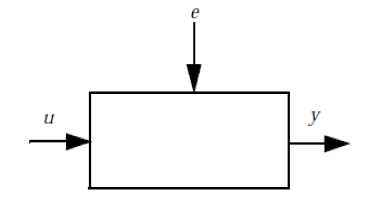
Fig.7. Input-Output Configuration

To ARX modeling three factors are important: inputs, noise and output. Figure 7 shows the basic input-output configuration [12-15].

Assuming the signals are related by a linear system, the relationship can be written y (t) = G (q )U (t) + e (t)

where q is the shift operator and G(q).U(t) is short for:

G(q)U(t)=∑g(k).U(t-k)(6)

and

G(q)=∑g(k)q ,q u(t)=u(t-1)(7)

The parameters of the ARX model structure is:

A(q)y(t) = B(q) u(t) + e(t)(8)

The order in ARX modeling is:

nn=[na nb nk](9)

Where na is output order in ARX, nb is input order in ARX and nc is delay order. The nn in ARX identification is [2 2 1].

Discrete-time IDPOLY model in ARX for step input is:

( )  ( ) =   ( )  ( ) +( )

( ) = 1 - 1․718    + 0․9048

( ) = 0․4839    - 0.4371

In this identification the, Loss function 6.51358-

031 and    6.68669-031

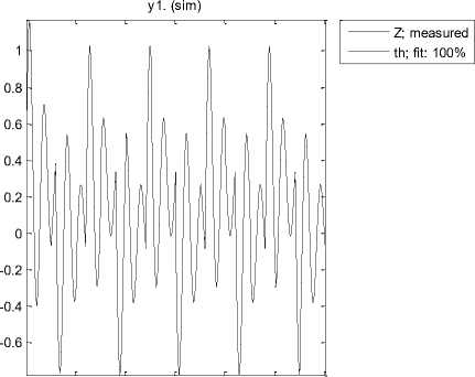
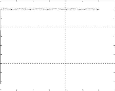
The fitting between input/output is 100% as Figure 8.

y1. (sim)

0.8

0.6

0.2

-0.2

50     100     150    200     250    300

Fig.8. Fitting test compare between ARX identification and output

Z; measured th; fit: 100%

Figure 9 shows the error between estimate identification system and real output.

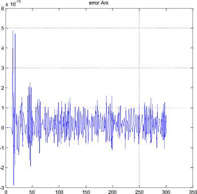
Fig.9. Error test compare between ARX identification and output

Discrete-time IDPOLY model ARX modeling for pulse input is:

л( q ) у ( t ) = В ( q ) и ( t ) + е ( t )

А ( q ) = 1 - 1.718 q ¹ + 0.9048 q"²

в ( q ) = 0.4839 q ¹ - 0.4371 q"²

Loss function 1.66081e-015 and FPE 1.70495e-015.

The fitting between input/output is 100% based on Figure 10.

50     100    150    200    250    300

Fig.10. Fitting test compare between ARX identification and output (Pulse input)

Figure 11 shows the error between estimate identification system and real output in pulse input.

Discrete-time IDPOLY model ARX modeling for ramp input is:

a ( q ) у ( t )= В ( q ) и ( t )+ e ( t )

A ( q ) = 1 - 1.718 q ¹ + 0.9049 q"²

в ( q ) = 0.4818 q ¹ - 0.4342 q"²

Loss function is 1.26637e-006 and FPE is 1.30003e-006.

The fitting between input/output is 99.11% based on Figure 12.

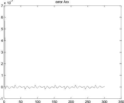
Fig.11. Error test compare between ARX identification and output in pulse input

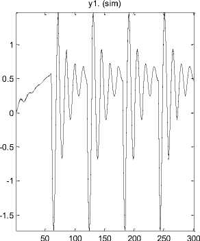
Fig.12. Fitting test compare between ARX identification and output (Ramp input)

Z; measured th; fit: 99.11%

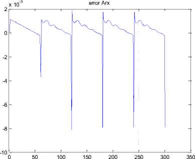
Fig.13. Error test compare between ARX identification and output in ramp input

Discrete-time IDPOLY model ARX modeling for band limited white noise input is:

л( q ) у ( t ) = В ( q ) и ( t ) + е ( t )

А ( q ) = 1 - 1.718 q ¹ + 0.9048 q"²

в ( q ) = 0.4839 q ¹ - 0.4371 q"²

Loss function is 2.25909e-016 and FPE is 2.31913e-016.

The fitting between input/output is 100% based on Figure 14.

y1. (sim)

Fig.14. Fitting test compare between ARX identification and output (Band limited white noise)

Z; measured th; fit: 100%

Figure 15 shows the error between estimate identification system and real output in band limited white noise input.

error Arx

-7 x 10-7

2.5

1.5

0.5

Fig.15. Error test compare between ARX identification and output in band limited white noise input

0       50       100      150      200      250      300      350

-0.5

Discrete-time IDPOLY model ARX modeling for input random numbers is:

A ( q ) у ( t ) = В ( q ) и ( t ) + e ( t )

A ( q ) = 1 - 1.718 q ¹ + 0.9048 q"²

в ( q ) = 0.4839 q ¹ - 0.4371 q"²

Loss function is 5.65716e-016 and FPE is 5.80752e-016.

The fitting between input/output is 100% based on Figure 16.

y1. (sim)

50    100    150    200    250    300

Fig.16. Fitting test compare between ARX identification and output (Input Random Number)

1.5

0.5

Z; measured th; fit: 100%

0.5

-4.5 0

Figure 17 shows the error between estimate identification system and real output in input random number test.

error Arx

-7 x 10^-7

-0.5

-1

-1.5

-2

-2.5

-3

-3.5

-4

50       100      150      200      250      300      350

Fig.17. Error test compare between ARX identification and output in input random number input

The Discrete-time IDPOLY ARMAX model is:

• a ( q ) у ( t ) = В ( q ) и ( t ) + c ( q ) e ( t )

0.5 s + 0.05

where

A ( q ) = 1 - 1.718 q ¹ + 0.9048 q"²

в ( q ) = 0.4839 q ¹ - 0.4371 q"²

c ( q )= 1 + 0.7278 q ¹+ q"²

Loss function 1.30582 е -027 and FPE 1.35822 е -027.

Based on ARX system identification the S domain transfer function and Z domain transfer functions are:

^Н(S)= s² +0.1 S +0.2

0.4839 Z - 0.4371

^Н(Z)= Z² - 1.7177 Z + 0.9048

• III. ARMAX System’S Identification

The general input-output form is:

A(q)y(t) = Б (( Б) u(t-nk)+Б (( Б ) e(t)(10)

The parameters of the ARMAX model structure is:

A(q)y(t) = B(q) u(t) + C(q)e(t)(11)

The order in ARMAX modeling is:

nn=[na nb nc nk](12)

Where na is output order in ARMAX, nb is input order in ARMAX, nc is the noise order and nk is the delay order and the nn in ARMAX identification is [2 2 1 1].

The Discrete-time IDPOLY ARMAX model for step input is:

А ( q ) у (t) = В ( q ) и (t) + с ( q ) е (t)

where

л( q ) = 1 - 1.718 q ¹ + 0.9048 q"²

в ( q ) = 0.4839 q ¹ - 0.4371 q"²

c ( q ) = 1 + 0.0336 q ¹ + 0.2794 q"²

y1. (sim)

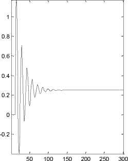
Fig.18. Fitting test compare between ARMAX identification and output

Z; measured th1 rmax; fit: 100%

Loss function 6.20333 e -031 and FPE 6.45653 e -

The fitting between input/output is 100% as Figure 18.

Figure 19 shows the error between estimate identification system and real output in ARMAX modeling.

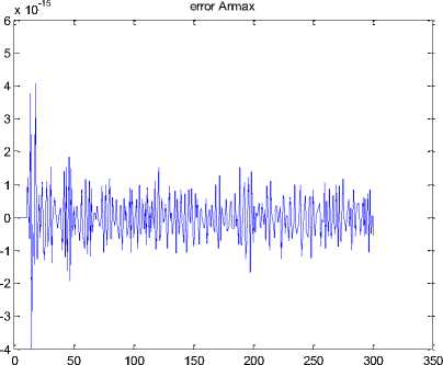
Fig.19. Error test compare between ARMAX identification and output

Regarding to final predictive error (FPE) for ARX and ARMAX in step input, ARMAX modelling is better than ARX in this type of input.

The Discrete-time IDPOLY ARMAX model for pulse input is:

A ( q ) у ( t ) = В ( q ) и ( t ) + c ( q ) e ( t )

where

A ( q ) = 1 - 1.718 q ¹ + 0.9048 q"²

в ( q ) = 0.4839 q ¹ - 0.4371 q"²

c ( q ) = 1 + 0.6501 q ¹+ q"²

Loss function 1.48899 e -027 and FPE 1.54875 e -027.

The fitting between input/output is 100% for pulse input ARMAX modeling shows in Figure 20.

50   100   150   200   250   300

Fig.20. Fitting test compare between ARMAX identification and output (pulse input)

Z; measured th1 armax; fit: 100%

Figure 21 shows the error between estimate identification system and real output in ARMAX modeling in pulse modeling.

identification system and real output in ARMAX modeling in ramp modeling.

x 10-7

error Armax

-1

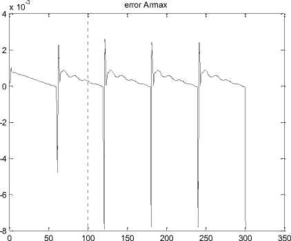
Fig.23. Error test compare between ARMAX identification and output in ramp input

Fig.21. Error test compare between ARMAX identification and output in pulse input

Regarding to final predictive error (FPE) for ARX and ARMAX in pulse input, ARMAX modelling is better. The Discrete-time IDPOLY ARMAX model for ramp input is:

Л( q ) у ( t ) = В ( q ) и ( t ) + с ( q ) е ( t )

where

А ( q ) = 1 - 1.717 q ¹ + 0.9045 q"²

в ( q ) = 0.481 q ¹ - 0.4336 q"²

c ( q ) = 1 + 0.2618 q ¹ + 0.1648 q"²

Loss function 1.19057 e -006 and FPE 1.23835 e -006. The fitting between input/output is 98.86% for ramp input ARMAX modeling shows in Figure 22.

Regarding to final predictive error (FPE) for ARX and ARMAX in ramp input, ARMAX modelling is better. The Discrete-time IDPOLY ARMAX model for band limited white noise is:

A ( q ) у ( t ) = В ( q ) и ( t ) + c ( q ) e ( t )

where

A ( q ) = 1 - 1.718 q ¹ + 0.9048 q"²

в ( q ) = 0.4839 q ¹ - 0.4371 q"²

c ( q )= 1 + q ¹ - 1.577 e -005 q"²

Loss function 7.36336 e -024 and FPE 7.65888 e -024.

The fitting between input/output is 100% for band limited white noise input ARMAX modeling shows in Figure 24.

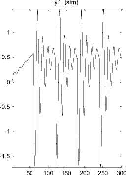
Fig.22. Fitting test compare between ARMAX identification and output (ramp input)

Z; measured th1 rmax; fit: 98.86%

Fig.24. Fitting test compare between ARMAX identification and output (band limited white noise input)

Z; measured th1 rmax; fit: 100%

Figure 23 shows the error between estimate

Figure 25 shows the error between estimate identification system and real output in ARMAX modeling in band limited white noise modeling.

_{x 10}^-7                         error Armax

• 3:----------------------------------с-----------------с-----------------с-----------------с-----------------с-----------------г

2.5

• 1.5

0.5

• -0.5 --------------------------£-------------£-------------£-------------£-------------£-------------1

0       50      100      150      200      250      300      350

• Fig.25. Error test compare between ARMAX identification and output in band limited white noise input

Regarding to final predictive error (FPE) for ARX and ARMAX in band limited white noise input, ARMAX modelling is better.

The Discrete-time IDPOLY ARMAX model input random number is:

Л( q ) у ( t ) = В ( q ) и ( t ) + с ( q ) е ( t )

where

А ( q ) = 1 - 1.718 q ¹ + 0.9048 q"²

в ( q ) = 0.4839 q ¹ - 0.4371 q"²

c ( q )= 1 + 0.7278 q ¹+ q "²

Loss function 1.30582 e -027 and FPE 1.35822 e -027 . The fitting between input/output is 100% for random numbers input ARMAX modeling shows in Figure 26.

y1. (sim)

50    100   150   200   250   300

Fig.26. Fitting test compare between ARMAX identification and output (random numbers input)

Z; measured th1 rmax; fit: 100%

Figure 27 shows the error between estimate identification system and real output in ARMAX modeling in random numbers input modeling.

_{x 10}^-7                          error Armax

0       50       100      150      200      250      300      350

0.5

-0.5

-1

-1.5

-2

-2.5

-3

-3.5

-4

-4.5

Fig.27. Error test compare between ARMAX identification and output in random numbers input

Regarding to final predictive error (FPE) for ARX and ARMAX in random numbers input, ARMAX modelling is better. Based on system ARMAX identification the S domain transfer function and Z domain transfer functions are:

0.5 s + 0.05 H ( s )=—

+0.1 +0.2

0.4839 z - 0.4371

^{H (z})= z² - 1.7177 Z + 0.9048

Table 1 shows ARX and ARMAX parameter identification in five types of inputs.

Table.1. System’s parameters Identification (ARX Vs ARMAX)

system	a1	a2	b1	b2	c1	c2
ARX Step	-1.718	0.9048	0.4839	-0.4371
ARMAX Step	-1.718	0.9048	0.4839	-0.4371	0.0336	0.2794
ARX Pulse	-1.718	0.9048	0.4839	-0.4371
ARMAX Pulse	-1.718	0.9048	0.4839	-0.4371	0.6501	1
ARX Ramp	-1.718	0.9049	0.4818	-0.4342
ARMAX Ramp	-1.717	0.9045	0.481	-0.4336	0.2618	0.1648
ARX White noise	-1.718	0.9048	0.4839	-0.4371
ARMAX White noise	-1.718	0.9048	0.4839	-0.4371	1	1.57e-5
ARX Random number	-1.718	0.9048	0.4839	-0.4371
ARMAX Random Number	-1.718	0.9048	0.4839	-0.4371	0.7278	1

• IV. Conclusion

Regarding to this research, system identification for highly nonlinear dynamic system (electric motor) is introduced. According to this research two methodologies are used for parameters identification: ARX modeling and ARMAX modeling. For data collection and data analysis, we have five types input-output regarding to this dynamic system. In final predictive error point of view, ARMAX modeling has better performance in comparison to ARX modeling. This methodology is important to design high performance controller for this electric motor.