Comparative Study of Krill Herd, Firefly and Cuckoo Search Algorithms for Unimodal and Multimodal Optimization

Published Online February 2014 in MECS

In recent times, nature inspired meta-heuristic algorithms are being widely used for solving optimization problems, including NP-hard problems which might need exponential computation time to solve in worst case scenario. In meta-heuristics methods [1, 9] we might compromise on finding an optimal solutions just for the sake of getting good solutions in a specific period of time. The main aim of meta-heuristic algorithms are to quickly find solution to a problem, this solution may not be the best of all possible solutions to the problem but still they stand valid as they do not require excessively long time to be solved. Two crucial characteristics of meta-heuristic algorithms are intensification and diversification. The intensification searches around the current best solution and selects the best candidate or solution. The diversification ensures that the algorithm explores the search space more efficiently. Maintaining balance between diversification and intensification is important because firstly we have to quickly find the regions in the large search space with high quality solutions and secondly not to waste too much time in regions of the search space which are either already explored or which do not provide high quality solutions [3].

In this paper, we have used three meta-heuristic algorithms Krill Herd Algorithm (KH) [4], Firefly Algorithm (FA) [1] and Cuckoo Search Algorithm (CS) [5].First is the Krill Herd Algorithm which was developed by Amir Hossein Gandomi and Amir Hossein Alavi in 2011. The KH algorithm is based on the simulation of the herding behaviour of Krill individuals. Second is the Firefly Algorithm (FA) which was developed by X.-S.Yang in 2007. It was inspired by the flashing pattern of fireflies. Third algorithm is the Cuckoo search Algorithm which was developed by X.-S.Yang and S.Deb in 2009. It is based on the interesting breeding behaviour of certain species of cuckoos such as brood parasitism.

This paper aims to provide the comparison study of the Krill Herd Algorithm (KH) with Firefly Algorithm (FA) and Cuckoo Search (CS) Algorithm via L´evy Flights against unimodal and multimodal test functions. Rest of the paper is organised as follows. First we will briefly explain the Krill Herd Algorithm, Firefly Algorithm, Cuckoo Search Algorithms and several Mathematical benchmark functions in section (II).Then experimental settings and results will be shown in section (III) and then finally we will conclude the paper.

• II.    Nature Inspired Algorithms and Optimization

• 2.1    Krill Herd Algorithm

  • 2.1.1    Krill Swarm’s Herding Behavior

• 2.1.2    Krill Herd Algorithm

Many Research have been done in order to find the mechanism that lead to the development non- random formation of groups by various marine animals

[11,12].The significant mechanisms identified are feeding ability, protection from predators, enhanced reproduction and environmental condition [6].

Krills from Antarctic region are one of the best researched marine animals. One of the most significant ability of krills is that they can form large swarms [13, 14].Yet there are number of uncertainties about the mechanism that lead to distribution of krill herd [15].There are proposed conceptual models to explain observed formation of krill heard [16] and result obtained from those models states that krill swarms form the basic unit of organization for this species.

Whenever predators (Penguins, Sea Birds) attack krill swarms, they take individual krill which leads in reducing the krill density. After the attack by predators, formation of krill is a multi- objective process mainly including two Goals: (1) Increasing Krill density and (2) Reaching food. Attraction of Krill to increase density and finding food are used as objective function which finally lead the krills to herd around global minima. In this mechanism, all individual krill moves towards the best possible solution while searching for highest density and food.

As Predator remove individual from Krill swarm, the average krill density and distance of krill swarm from the food location decreases. We assume this process as the initialization phase in the Krill Herd Algorithm [4]. Value of objective function for each individual is supposed to be combination of distance from food and highest density of krill swarm. Three essential actions [6] considered by Krills to determine the time dependent position of an individual krill are:

• (i)    Movement induced by other krill individuals

• (ii)    Foraging activity

• (iii)    Random Diffusion

• 2.1.3    Motion Induced by other krill individual

We know that all the optimization algorithm should have searching capability in space of arbitrary dimensionality. Hence we generalize Lanrangian model of krill herding to n dimensional decision space.

dXjdt =N_vVF_v-VD_t                   (1)

Here Л^г, is the motion induced by other krill individuals, Ff is the foraging motion and Of stands for physical diffusion for ith krill individuals.

According to research krill individuals move due to the mutual effects by each other so as to maintain high density [6].Movement for the krill individual is defined as:

N^” _ ^тмд. ₊ ^tf^               (2)

In (2) до-так stands for maximum induced speed which is equal to 0.01 (m/s) [6] , ^aL is the direction of motion induced which is estimated from target swarm density and local swarm density, ш_п is the inertia weight of the motion induced, IV °^ is the last motion induced.

a_t = a^l_t^Mal + a*"⁸®¹                           (3)

In (3) H^ is the local effect due to the neighbors, and         is the target direction effect due to the best krill individual.

Attractive or Repulsive effect of the neighbors on an individual krill movement can be formulated as:

^ = ^NM.(4)

Уй. = ^ - уукг - yJUf(5)

<7= ^i - К(/К"'огя - Kbsst(6)

In (4) NN is the number of the neighbors. In (5) and (6) I^WOTSt and _K=-3t are, the worst and the best fitness values of the krill individuals till now, A,^- represents the fitness value of the ith krill individual, ^f is the fitness of jth neighbor and X represents the related positions.

To choose the neighbor, using actual behavior of Krill individual, a sensing distance (ds) is calculated using d^ = l/S.V^Jkj - x, ||                 (7)

In (7) ^3 i is the sensing distance for the ith krill individual and N stands for number of krill individuals. Based on (7), two krill individuals are neighbor if the distance between them is less than G.

The effect of the individual krill having the best fitness on the ith individual krill is calculated as follow:

target _ „ best S у

In (8) _coest is the effective coefficient of the krill with the best fitness and is defined as:

C^ = 2 (rand + I/I^              (9)

Where rand is a random value in the range [0, 1], I is the actual iteration number, and Imax is the maximum number of iterations.

• 2.1.4    Foraging motion

Foraging motion is developed in terms of two main effective parameters. One is the food location and the second one is the previous experience about the food location. This motion can be explained for the ith krill individual as follow:

^ = V_fp_t + c^                   (10)

Where

Pi = ^+^             (11)

In (10) Vf is the foraging speed, •^f is the inertia weight of the foraging motion in the range [0, 1] and F^^d is the last foraging motion. In (11) pfood and p^^st are the food attractive effect and best fitness of the ith krill so far respectively. Measured values of the foraging speed [7] is 0.02( ms ~ ).

The center of food is found at first and then food attraction is formulated. The virtual center of food concentration is estimated according to the fitness distribution of the krill individuals, which is inspired from ‘‘center of mass’’. The center of food for each iteration is formulated as:

xf00d = ^ 1/К( Xi ^ VKt(12)

Hence, we can evaluate the food attraction for the ith krill individual by following equation:

In (13) (•food is the food coefficient. As time passes the effect of food in the krill herding decrease and food coefficient is evaluated as:

Cfood = 2(1 _ in^(14)

The attraction towards food is defined to attract the krill swarm towards global optima. Based on this definition, the krill individuals normally herd around the global optima after some iteration. This can be considered as an efficient global optimization strategy which helps improving the global optima of the KH algorithm.

The effect of the best fitness of the ith krill individual is also handled using the following equation:

Pi ^— ^iibest^iibest                          (15)

In (15) Ffoest is the best previously visited position of the ith krill individual.

• 2.1.5    Physical diffusion

• 2.1.6    Motion Process of the KH Algorithm

The physical diffusion of all the krills is basically a random process. We can express this motion in terms of maximum diffusion speed and a random directional vector. We can formulate it as follows:

D_t = D™“6                            (16)

In (16) j^max is the maximum diffusion speed [8] and 6 is the random directional vector and it includes random values in range [-1, 1]. As krills position gets better, random motion is also reduced. Thus, another term is added to the physical diffusion formula to consider this effect. The effects of the motion induced by other krill individuals and foraging motion gradually decrease increase in iterations. The physical diffusion is a random vector hence it does not steadily reduces with increase in number of iterations due to which another term is added to (16). This term, linearly decreases the random speed with time and works on the basis of a geometrical annealing schedule:

Di = D™^(1- 1/1^6               (17)

The defined motions frequently change the position of a krill individual toward the best fitness. The foraging motion and the motion induced by other krill individuals contain two global and two local strategies. KH a powerful algorithm as all these work in parallel. The formulations of these motions for the ith krill individual show that, if fitness value of each of the above mentioned effective factor like K-; , _Kb_$st , _KfOQd , _Kp=t is better i.e. less than the fitness of the ith krill, it has an attractive effect else it is a repulsive effect. We can notice from the above formulations that better fitness has more effect on the movement of ith krill individual. The position vector of a krill individual during the interval t to t + Дt is given by the following equation:

Xi (t + At) = Xi (t) + At dXi /dt               (18)

Д t should be carefully set according to the optimization problem because this parameter works as a scale factor of the speed vector. Дt completely depends on the search space and it can be obtained simply by the following formula:

At=C_ty.^(UBi-LBi)                (19)

In (19) NV is the total number of variables and LB.; and UE; are lower and upper bounds of the jth variables respectively. It is empirically found that C -is a constant number between [0, 2]. Lower the values of C_f more carefully the krill individuals will search.

• 2.1.7    Crossover

• 2.2    Firefly Algorithm

  • 2.2.1    Behavior and nature of Fireflies

• 2.2.2    Firefly Algorithm

To improve the performance of the algorithm, genetic reproduction mechanisms are incorporated into the algorithm. One such algorithm is crossover. Crossover is a genetic operator used to vary the programming of chromosomes from one generation to the next. In this Algorithm, an adaptive vectored crossover scheme is employed.

We can control crossover by a crossover probability , Ст , and actual crossover can be performed in two ways: binomial and exponential. The binomial scheme performs crossover on each of the d components or variables/parameters. By generating a uniformly distributed random number between 0 and 1, the mth component of X,; , ^Х1ТП, is determined as:

Cr = 0.2K_ibest (21)

In (20) r E {1, 2,. . ., i _ 1, i + 1,. . .,N}. With this new crossover probability, the crossover probability for the global best is equal to zero and it increases with decrease in fitness.

Fireflies are the creatures that can generate light inside of it. Light production in fireflies is due to a type of chemical reaction. The primary purpose for firefly’s flash is to act as a signal system to attract other fireflies. Although they have many mechanisms, the interesting issues are what they do for any communication to find food and to protect themselves from enemy hunters including their successful reproduction. There are around two thousand firefly species, and most of them produce short and rhythmic flashes. The pattern observed for these flashes is unique specific species. The rhythm of the flashes, rate of flashing and the amount of time for which the flashes are observed together forms a pattern that attracts both the males and females to each other. Females of a species respond to individual pattern of the male of the same species.

The light intensity at a particular distance from the light source follows the inverse square law. That is as the distance increases the light intensity decreases. Furthermore, the air absorbs light which becomes weaker and weaker as there is an increase of the distance. There are two combined factors that make most fireflies visible only to a limited distance that is usually good enough for fireflies to communicate each other. The flashing light can be formulated in such a way that it is associated with the objective function to be optimized. This makes it possible to formulate new meta-heuristic algorithms.

The firefly (FA) algorithm [1, 9, 10] is a meta heuristic algorithm, inspired by the flashing behavior of fireflies. The primary purpose for a firefly's flash is to act as a signal system to attract other fireflies.

Xin-She Yang formulated this firefly algorithm by taking three assumptions [1]

• i.    All fireflies are unisexual, so that one firefly will be attracted to all other fireflies;

• ii.    Attractiveness is proportional to their brightness, and for any two fireflies, the less bright one will be attracted by (and thus move to) the brighter one; however, the brightness can decrease as their distance increases;

• iii.    If there are no fireflies brighter than a given firefly, it will move randomly.

• 2.2.3    Light Intensity and Attractiveness

Two core issues in firefly algorithm are (i) The variation of light intensity, (ii) The formulation of the attractiveness.

For simplicity, it is assumed that the attractiveness of a firefly is determined by its brightness which in turn is associated with the encoded objective function of the optimization problems. In the simplest case for maximum optimization problems, the brightness I of a firefly for a particular location x could be chosen as I(x) ∝  f(x). Even so, the attractiveness β is relative, it should be judged by the other fireflies. Thus, it will differ with the distance 4j between firefly i and firefly j. In addition, light intensity decreases with the distance from its source, and light is also absorbed by the media, so we should allow the attractiveness to vary with the varying degree of absorption.

Since a firefly’s attractiveness is proportional to the light intensity seen by adjacent fireflies, attractiveness β of a firefly can be defined as

^(r) = ров-^ , (m≥1),               (22)

In (22), r or ^ is the distance between the ith and jth fireflies. Pq Is the attractiveness at r = 0 and γ is a fixed light absorption coefficient. The distance between any two fireflies ith and jth at ^XL and Xj is the Cartesian distance and can be calculated as:

T_tj = Ik - x_;|| = J^₌₁(x_tjt-X_j;it)² (23)

In (23), ^ii is the k th component of the i th firefly (^ZL). The movement of ith firefly, to another more attractive (brighter) jth firefly, is determined by

xt = х, + poe">yy(xj- Xi) + a(rand -0.5) (24)

In (24) the second term is due to the attraction while the third term is the randomization with α being the randomization parameter. Rand is a random number generator uniformly distributed in the range of [0, 1]. For most cases in the implementation, 0_C = 1 and α ∈ [0, 1]. Furthermore, the randomization term can easily be extended to a normal distribution N (0, 1) or other distributions.

• 2.3    Cuckoo Search Algorithm via Lévy Flight

  • 2.3.1    Cuckoo’s breeding behavior

• 2.3.2    Lévy flight

• 2.3.3    Cuckoo Search Algorithm

Cuckoo is an interesting bird species, known not only for the beautiful sound they make, but also for their aggressive reproductive strategy. Cuckoos are extremely diverse group of birds with regards to breeding system. Many Cuckoo species follow the strategy of brood parasitism by using host individuals either of the same or different species to raise the young of the own. Cuckoo species such as Anis and Guira lay their eggs in communal nest though they may remove others eggs to increase the survival probability of their own eggs. Some host birds can engage in direct conflict with the intruding cuckoos. On recognition of parasitic eggs, the host may kick the parasites eggs out, or build a new nest. Female parasitic cuckoos who are specialized in mimicry lay eggs that closely which resemble the eggs of their host which reduces the probability of their eggs being abandoned.

Parasitic cuckoos often choose a nest where host bird have just laid their eggs .The cuckoo egg hatches earlier as compared to the host's, and the cuckoo chick grows faster than them;. In most cases the chick evicts the eggs laid by host species, which increases the cuckoo chick’s share of food provided by its host bird. Some cuckoo chick can even replicate the call of host chicks to gain access to more feeding opportunity.

A Lévy flight is a random walk in which the steplengths have a probability distribution that is heavytailed. Research works have shown that flight behavior of many animals and insects demonstrated the typical characteristics of Lévy flights [17, 18, 19, 20]. Fruit flies or Drosophila melanogaster, explore their landscape using a series of straight flight paths punctuated by a sudden 90 degree turn, leading to a Lévy -flight-style intermittent scale free search pattern was shown in a study conducted by Reynolds and Frye. Many researches shows that Lévy flights interspersed with Brownian motion can describe the animals' hunting patterns [24, 25]. Even light can be related to Lévy flights [23]. Latterly, such behavior has been applied to optimization and optimal search, and preliminary results show its promising capability [18, 20, 21, 22].

Each egg in the nest represents solution, and Cuckoo egg represents new solution. The aim is to use the new and potentially better solutions (Cuckoos) to replace not-so-good or inferior solution in the nests. In the simplest form, each nest has one egg. The algorithm [5] can be extended to more complicated cases in which each nest has multiple eggs representing a set of solutions.

Cuckoo search is based on three idealized rules which states that

• i.    Each Cuckoo lays one egg, which represents a set of solution coordinates, at a time, and dumps it in a random nest.

• ii.    A fraction of the nests containing the best eggs, or solutions, will be carried over to the next generation.

• iii.    The number of nests is fixed and there is a probability that a host can discover an alien egg. If this happens, the host can either discard the egg or the nest and this result in building a new nest in a new location.

2.4 Testing Optimization Functions

When generating new solutions JC^C+" for the ith Cuckoo, Lévy Flight is performed.

xf = xf+1 + a©Levy(Jl)                    (25)

In (25), α > 0 is the step size which should be related to the scales of the problem of interest. In most cases, we can use α = O (L/10) where L is the characteristic scale of the problem of interest. The above equation is essentially the stochastic equation for a random walk. The product ⊕ means entry wise multiplications.

The Lévy flight essentially provides a random walk whose random step length is drawn from a Lévy distribution

Levy "u = t^-;- , О. < л < 3)           (26)

This has an infinite variance with an infinite mean. Here the steps essentially form a random walk process with a power-law step-length distribution with a heavy tail. Some of the new solutions should be generated by Levy walk around the best solution obtained so far, this will speed up the local search. To ensure that that the system will not be trapped in a local optimum, a substantial fraction of the new solutions should be generated by far field randomization whose locations should be far enough from the current best solution.

In Literature [26] there are many benchmark test functions which are designed to test the performance of optimization algorithms. In this paper we will compare and validate above mentioned algorithms against these benchmark functions. Seventeen functions [27,28,29] including many multimodal functions are used in this paper in order to compare and verify efficiency and convergence of all three above mentioned Nature Inspired Algorithms. Certain test functions used in our simulations are as follows:

Ackley Function is multimodal function widely used for testing optimizat1ion algorithms.

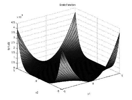
Fig. 2: The visualization of the Beale function

f(x) = -20 exp

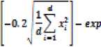
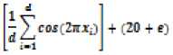
With a global minimum fU.) = о at xe = (0,0......0) in the range of xi ∈ [-32.768, 32.768], for all i = 1, 2… d.

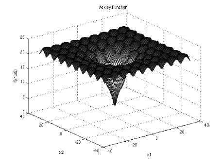
Fig.1: The visualization of the Ackley function

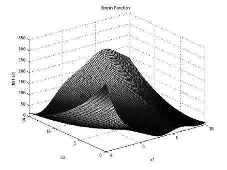
Fig. 3: The visualization of the Branin function

Colville is a unimodal test function.

Beale function is 2- dimensional multimodal function, with sharp peaks at the corners of the input domain.

/(x) = (1.5 - z, + z^)2 4 (2.25 - zt - z^2 + (2.625 - z, + z,^)1

Which has minimum /(x.) = 0, at x„ = (3,0.5) in range ^xi ∈ [-4.5, 4.5], for all i = 1, 2.

Branin function is multimodal with three global minima. The recommended values of a, b, c, r, s and t are: a = 1, b = 5.1 ⁄ (4π2), c = 5 ⁄ π, r = 6, s = 10 and t = 1 ⁄ (8π).

/(x) = a(z₅ - bx^ + ci| — r)² + s(l — t)coe(z|) 4- s

With a global minimum f(xj = 0.397887 at x. = (-x, 12.275), U. 2.275) and (9.42478,2.475 in the range ^xi ∈ [-5, 10] and x2 ∈ [0, 15].

Which has minimum f(x.) = O.atx. = (1,1,1,1) in range ^xi ∈ [-10, 10], for all i = 1, 2, 3, 4.

Dixon-Price’s unimodal test function

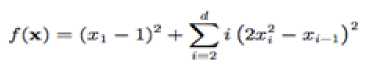
With a global minimum f(x.) = 0

at xt = 2

bin the range of ^xi ∈ [-10, 10], for all i = 1, 2… d.

Easom function has several local minima. It is unimodal, and the global minimum has a small area relative to the search space.

/(x) = -coe(xi) coe(x2) exp (—(Xi — я)2 — (x2 — я1)3)

Which has minimum f (x.) = —l,at x. = (^тг) in range Xf ∈     [-100,100], for all i =   1,  2,

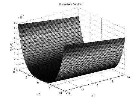
Fig. 4: The visualization of the Dixon-Price’s function

Fig. 5: The visualization of the Easom function

Shubert function a multimodal test function has several local minima and many global minima. Its equation is

Which has minimum f^J = -186.7309, in range

Z[ ∈ [-10, 10], for all i = 1, 2,

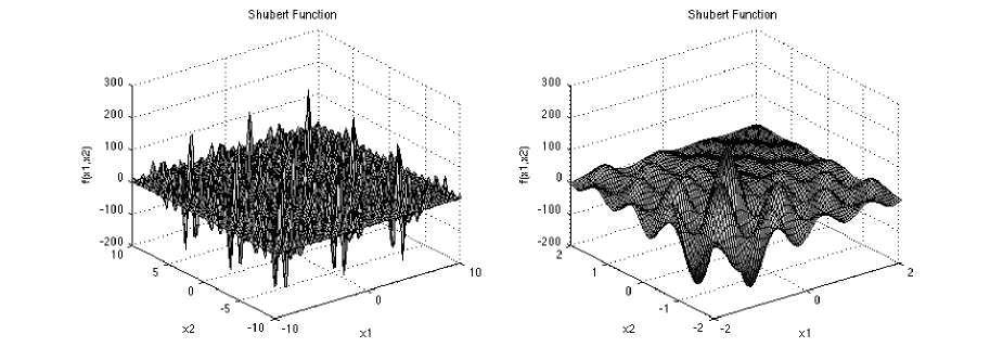
Fig. 6: The visualization of the Shubert function

Levy Test function is multimodal function. Its equation is d-1

fW = ^(пГ1)-ь^(г,-1)* [1 ♦ 10s33(rr, +1)] + (r<-lf [1 + sa'IZn^)], where e, ■ 1 +      , for all i ■ lf...,d

With a global minimum f Or.) = о at -i = Ci.....i) which is evaluated in the range of ^XL ∈ [-10, 10], for all : = 1, 2… d.

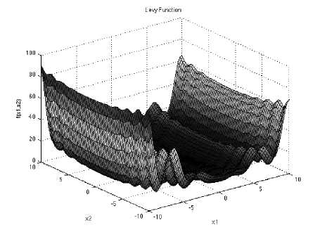
Fig. 7: The visualization of the Levy function

Rastrigin function has several local minima. It is highly multimodal, but locations of the minima are regularly distributed.

d

/(x) = 10d + У^ [z? — 10cos(2irr,)]

With a global minimum fUJ = о at x. = (0,0......0) evaluated in the range of ^xi ∈ [-5.12,

5.12], for all : = 1, 2… d.

Fig. 8: The visualization of the Rastrigin function

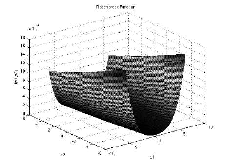
Fig. 9: The visualization of the Rosenbrock function

Rosenbrock function is unimodal, and the global minimum lies in a narrow, parabolic valley.

/(x) - У2 [1ОО(®« t - x?)³ + (Zi - I)³] t-1

With a global minimum f Or.) = о at ^xi = (l.....1) which is evaluated in the range of ^XL ∈ [-5, 10], for all : = 1, 2… d.

Zakharov function has no local minima except the global one. It’s a unimodal function and its equation is

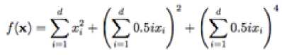
With a global minimum f Or.) = 0 at xi = (0.....0)

which is evaluated in the range of ^XL ∈ [-5, 10], for all := 1, 2… d.

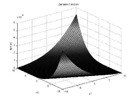
Fig. 10: The visualization of the Zakharov function

Griewank function has many widespread local minima, which are regularly distributed. It is a multimodal test function.

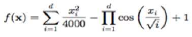
With a global minimum f Or.) = 0 at xi = (0.....0)

which is evaluated in the range of ^XL ∈ [-600, 600], for all i = 1, 2… d.

Grlevank Function

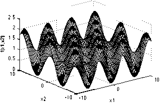
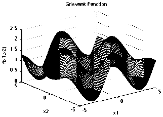
Fig. 11: The visualization of the Griewank function

Trid function has no local minimum except the global one. It is a unimodal function.

/(х) = ^(Xi - I)² - ^Z.r. l <•1              i-2

With a global minimum fU.) = -50 for d=6 and f (r.) = -200 at d=10 which is evaluated in the range of ^xi ∈ [-d², d¹ ], for all : = 1,2, …, d.

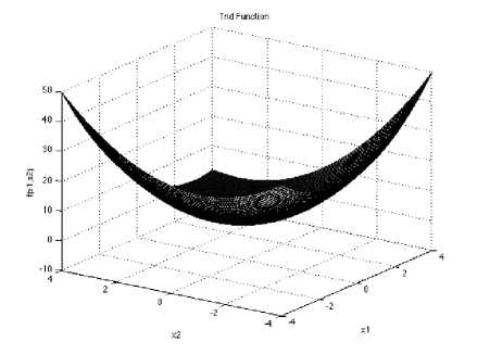
Fig. 12: The visualization of the Trid function

Powell Function is a unimodal function

/(x) * Z [I8*-1 * ^-l)1 * ^«-l ■ *•)**(*•-• ■ ^ ■>* * MK*»-»* *»)*)

This function is usually evaluated on the region x i ∈ [-4, 5], for all i = 1, 2… d. having minima f Or.) = 0 at х_£ = (3,-1,0,1.....3.-1.0)

Eggholder function is a difficult function to optimize, because of the large number of local minima. It is multimodal test function.

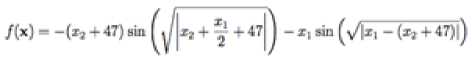
Which            has            minimum

f(xj = —959.6407, at x. = (512,404.2319) in range

^XL ∈ [-512, 512], for all i = 1, 2.

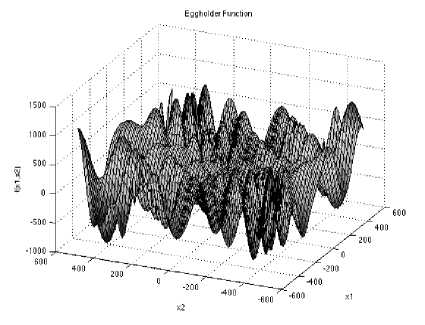
Fig. 13: The visualization of the Eggholder function

• III.    Implementation and Numerical Experiments

  In this section we will compare the performance of Krill Herd algorithm Firefly algorithm, Cuckoo search algorithm for various benchmark test functions. The benchmarks function include both unimodal and multimodal with both low and high dimensional problems are described in Section 2.4 and for evaluation all computational procedures described above has been implemented in MATLAB™ computer program. In order to compare these algorithms we have carried out extensive simulations and each algorithm has been run 50 times so as to carry out meaningful analysis. The maximum number of function evaluations is set as 10,000 for high dimensional functions and 1000 for low dimensional functions.

• 3.1    Optimization for Unimodal Test Function

• 3.1.1    Optimization fitness

Here for Krill Herd Algorithm С" 7 is set to 0.5 and the inertia weights (&)_R, to^ ) are equal to 0.9 at beginning of search and it linearly decreases to 0.1 at the end. For Firefly algorithm certain constants are fixed as a = 0.5, p = 0.2 and у = 1 for simulation. For cuckoo search algorithm probability for host bird is fixed as и, = O'.25. For simulation we have used various population sizes from n = 10 to 150, and found that for most problems, it is sufficient to use n = 15 to 50. Therefore, we have used a fixed population size of n = 50 in all our simulations for comparison.

Now we will divide this section in two parts comprising comparison of algorithms for unimodal test function in first section and comparison of algorithms for multimodal test functions in another. For both the section we will be comparing KH algorithm, FA Algorithm and CS Algorithm via Lévy Flights on the basis of three criteria i.e. Optimization fitness (efficiency), Convergence and processing time.

In this section we have compared KH algorithm, FA Algorithm and CS Algorithm via Lévy Flights on Eight Unimodal benchmark functions popular for optimization. Unimodal functions are those function which have only single local minima and these function easier to optimize.

Here we have calculated the mean fitness value using the above mentioned algorithms for all unimodal test functions mentioned above. Optimized fitness result where global optima is reached are summarized in Table 1.

Table 1: Comparison of Optimization Fitness for Unimodal Test Functions

Function/Algorithms	KH Algorithm	FFA Algorithm	CS Algorithm
Dixon-Price(d=20)	0.6975	0.6668	0.6667
Rosenbrock (d =20)	31.89	14.49	2.63e-14
Zakharov (d =20)	5.973	3.19e-06	2.77e-28
Powell (d =20)	0.0299	0.002269	5.27e-09
Trid (d =20)	9.34e+2	1.52e+03	1.52e+03
Beale	2.92e-11	5.49e-10	1.34e-30
Easom	-0.96	-0.86	-1
Colville	-1.40e+09	-1.56e+07	-7.57e+17

Here we can see that Cuckoo Search algorithm has outperformed both Krill Herd and Firefly algorithm. For all Unimodal test function, fitness value of CS algorithm is much closer to global optima as compared to other two algorithms. But if we just compare the other two algorithms i.e. Firefly and Krill herd algorithm, their result are very close to each other, but on average, results obtained using Firefly algorithm are slightly better than results obtained using Krill Herd algorithm. As per results from Table 1 it is visible that performance of Krill Herd algorithm is better for low dimensional functions and as we move from low dimensional function to high dimensional functions fitness value for krill herd decreases i.e. distance from global minima increases. According to results in Table 1 performance of Firefly algorithm is better than Krill

Herd algorithm for high dimensional functions but for low dimensional function result using Krill Herd algorithm are better than Firefly algorithm. Also in Krill Herd algorithm we have varied dimensions from d= 5 to 20 and observed that as we increases the dimensions, fitness value for function decreases.

• 3.1.2    Processing time

• 3.1.3    Convergence

Here we will compare above mentioned algorithms on basis on processing time. Processing time is basically time consumed by algorithm to process single simulation. It includes time consumed by fixed number of iteration to solve the problem.

Table 2: Comparison of processing time in seconds for Unimodal Test Functions

Function/Algorithms	KH Algorithm	FFA Algorithm	CS Algorithm
Dixon-Price (d =20)	141.73	125.56	19.69
Rosenbrock (d =20)	137.18	123.44	21.58
Zakharov (d =20)	137.66	125.66	22.92
Powell (d =20)	172.44	138.95	63.35
Trid (d =20)	155.12	146.04	30.72
Beale	13.034	11.18	1.64
Easom	12.69	12.13	2.46
Colville	13.33	12.92	2.59

From Table 2 it is quite easily visible that time taken or consumed by Cuckoo search algorithm is much less than the other two algorithms We can also compute from the Table 2 that time consumed by Firefly algorithm is less than Krill Herd Algorithm although difference is not much, In term of processing time Cuckoo search algorithm again outperform other two algorithms.

In this section convergence plots of the benchmark functions for three different algorithm i.e. Krill Herd,

Firefly, Cuckoo Search are compared for fixed number of iteration i.e. 10,000 iterations for high dimensional function and 1000 iteration for low dimensional function. Here we will estimate which algorithm gives potentially better and quicker convergence towards optimality. Below In Figure 14-21 Convergence Graph is plotted for all above mentioned Unimodal benchmark functions.

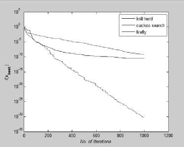
Fig. 14: Convergence Plot for Beale Function

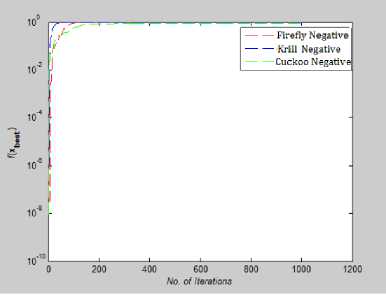
Fig. 18: Convergence Plot for Easom Function

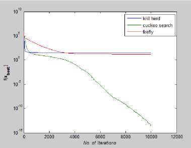
Fig. 15: Convergence Plot for Rosenbrock Function

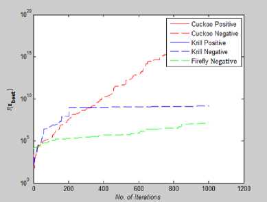
Fig. 19: Convergence Plot for Colville Function

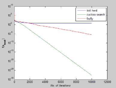
Fig. 16: Convergence Plot for Zakharov Function

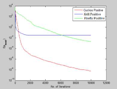
Fig. 20: Convergence Plot for Powel Function

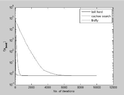
Fig. 17: Convergence Plot for Dixon-Price Function

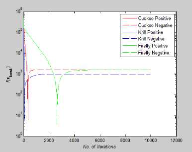
Fig. 21: Convergence Plot for Trid Function

Comparative Study of Krill Herd, Firefly and Cuckoo

Search Algorithms for Unimodal and Multimodal Optimization

In Fig.18, Fig.19 and Fig.21 we have plotted the absolute value of the fitness function. For Trid, Easom, Colville function, value of global minima is negative and so to plot them on convergence graph we took their absolute vale.

From Fig 14-21 we can interpret that the algorithm that quickly converges to its optimal solution is Krill Herd Algorithm. When we compare them on the number of iteration, Krill Herd Algorithm takes least number of iteration to converge whereas solution of other two algorithm are better in terms of fitness value. It can also be seen from Fig. 14-21 that for most of the test functions, the other two algorithms i.e. Firefly Algorithm and Cuckoo search algorithm do not converge till 10,000 iterations and for functions for which these two algorithm converges before 10,000 iterations, it is the cuckoo search algorithm which converges quickly than firefly for more of function as compare to number of function for which firefly algorithm converges faster than cuckoo search algorithm.

• 3.2    Optimization for Multimodal Test Function

• 3.2.1    Optimization fitness

In this section we have compared KH algorithm, FA Algorithm and CS Algorithm via Lévy Flights on Seven Multimodal benchmark functions popular for optimization. Multimodal functions are those function which have many number local minima and these function comparatively more difficult to optimize.

Here we have calculated the mean fitness value using the above mentioned algorithms for all multimodal test functions mentioned in Section 2.4. Optimized fitness result where global optima is reached are summarized in Table 3.

Table 3: Comparison of Optimization Fitness for Multimodal Test Functions

Function/Algorithms	KH Algorithm	FFA Algorithm	CS Algorithm
Ackley (d =20)	1.19e-05	7.36e-03	4.44e-15
Levy (d =20)	0.066	2.28e-06	1.14e-06
Rastrigin (d =20)	8.69	20.36	2.84
Griewank (d =20)	1.37e-09	5.89e-04	0
Branin	0.3979	0.3981	0.3981
Shubert	-186.7309	-186.7309	-186.7309
Eggholder	-893.0205	-930.2513	-959.6407

From Table 3 we can see that Cuckoo Search algorithm has outperformed both Krill Herd and Firefly algorithm in multimodal optimization as well. For all Multimodal test function, fitness value of CS algorithm is much closer to global optima as compared to other two algorithms. But if we together compare the other two algorithms i.e. Firefly and Krill herd algorithm for multimodal test functions, result for them are in contradiction with results in previous section for unimodal test functions. In multimodal optimization for most of the low dimensional function ,result for both the algorithms are almost equivalent, for most of the time both are able to find the global optima but for high dimensional multimodal functions fitness value obtained using Krill Herd is better than fitness value obtained using Firefly Algorithm. Results in Table 3 are in contradiction with results in Table 1 as in unimodal test function optimization fitness for high dimensional function using firefly was better than krill herd but in multimodal function optimization fitness using krill herd algorithm is better than firefly algorithm for high dimensional function.

Table 4: Comparison of processing time in seconds for Multimodal Test Functions

Function/Algorithms	KH Algorithm	FFA Algorithm	CS Algorithm
Ackley (d =20)	138.06	123.49	24.78
Levy (d =20)	169.37	129.03	38.86
Rastrigin (d =20)	139.55	126.31	24.58
Griewank (d =20)	137.18	123.44	21.58
Branin	13.36	11.28	1.91
Shubert	13.83	11.33	2.56
Eggholder	13.04	11.23	2.83

• 3.2.2    Processing time

• 3.2.3    Convergence

  Here convergence plots of the benchmark functions for three different algorithm i.e. Krill Herd, Firefly, Cuckoo Search are compared for fixed number of iteration i.e. 10,000 iterations for high dimensional function and 1000 iteration for low dimensional functions. Here we will estimate which algorithm gives potentially better and quicker convergence towards optimality. Convergence Graph for all above mentioned Multimodal benchmark functions are plotted in Figure 22-28.

In this section we will compare Krill Herd, Firefly, Cuckoo Search algorithms on basis on processing time for multimodal optimization functions. Processing time is basically time consumed by algorithm to process single simulation. It includes time consumed by fixed number of iteration to solve the problem.

Results in Table 4 are quite similar with the results in Table 2. In multimodal optimization function as well, time taken or consumed by Cuckoo search algorithm is much less than the other two algorithms It can also be interpreted from the Table 4 that time consumed by Firefly algorithm is less than Krill Herd Algorithm although difference is not much, In term of processing time Cuckoo search algorithm again outperform other two algorithms.

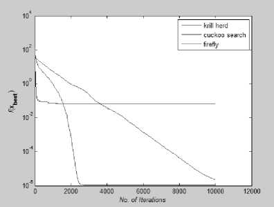
Fig. 24: Convergence Plot for Levy function

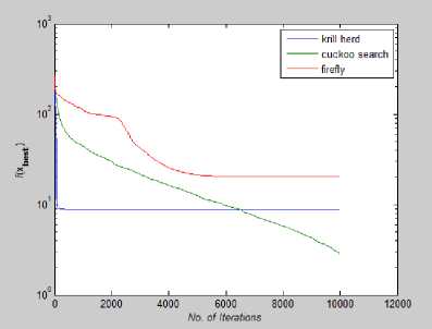
Fig. 25: Convergence Plot for Rastrigin Function

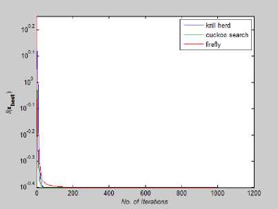
Fig. 22: Convergence Plot for Branin Function

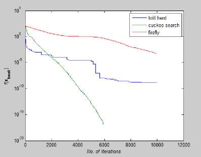
Fig. 26: Convergence Plot for Griewank Function

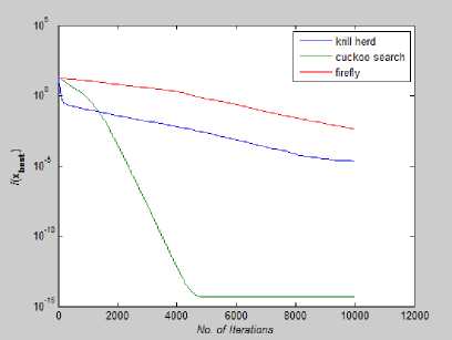
Fig. 23: Convergence Plot for Ackley Function

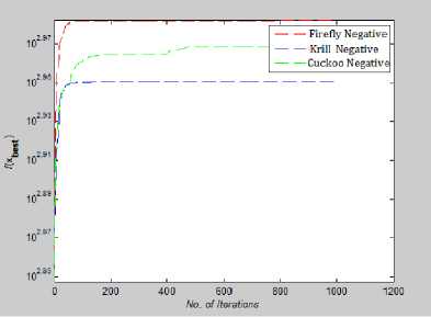
Fig. 27: Convergence Plot for Eggholder Function

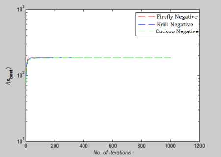
Fig. 28: Convergence Plot for Shubert Function

In Fig.27, and Fig.28 we have plotted the absolute value of the fitness function. In multimodal optimization Shubert and Eggholder function value of global minima is negative and so to plot them on convergence graph we took their absolute vale.

From Fig 22-28 we can interpret that although for many function all the algorithms are not able to converge before 10,000th iteration but for test functions like Rastrigin, Branin, Griewank, Levy and Eggholder, Krill herd algorithm is the fastest to converge to its optimal solution. When we compare them on the number of iteration, Krill Herd Algorithm takes least number of iteration to converge. If we see Fig.23 it is visible that for Ackley function Cuckoo Search Algorithm is the fastest to converge to its optimal solution others are not able to converge before 10,000th iteration. Also in Fig. 24 Cuckoo Search Algorithm is second fastest after Krill Herd algorithm to converge. From Fig 22-28 we can interpret that Firefly algorithm don not converge to its optimal solution for any of the high dimensional functions till 10,000th iteration. For multidimensional functions it is the Krill herd algorithm which is fastest to converge to its optimal solution, then after Krill Herd algorithm it is cuckoo search algorithm to converge to its optimal solution and at last is Firefly algorithm.

• IV.    Conclusion

In this paper we have compared latest meta-heuristic algorithms such as Krill Herd Algorithm, Firefly Algorithm and Cuckoo Search algorithm via Lévy Flights on basis of three criteria i.e. optimization fitness (efficiency), time processing and convergence. Results obtained by simulation of theses algorithms on unimodal and multimodal test functions shows that Cuckoo search algorithm is superior for both unimodal and multimodal test function in terms of optimization fitness and time processing whereas when comparison comes down to line between Krill Herd Algorithm and Firefly Algorithm, KH Algorithm is superior than FFA algorithm for multimodal optimization of both high and low dimensional functions whereas for unimodal optimization FFA algorithm is superior than KH Algorithm for High dimensional function but KH algorithm is superior for low dimensional functions but in terms of time processing FFA Algorithm is surpasses KH Algorithm for both unimodal and multi modal optimization. When we compare these algorithms on basis of convergence Krill Herd is the fastest of all to converge to its optimal solution after which comes the Cuckoo search algorithm and at last comes the Firefly algorithm which do not converge for most of the function to it optimal solution.

During simulation we also noticed that as we increase the dimension, fitness value or optimization fitness for KH algorithm decreases although it outperformed FFA algorithm for high dimensional multimodal function but on average as dimension increases optimization fitness for KH algorithm decreases.

As all these powerful optimization strategy are able to optimize both unimodal and multimodal test function effectively hence we can easily extend them to study multi objective optimization applications with various constraints and even to NP-hard problems.