Comparative Weka Analysis of Clustering Algorithm's

Published Online August 2017 in MECS

Recently, the generation and collection of data for various purposes had increased rapidly. Commercial sites, business sites, government sites, bank transaction, scientific and engineering field, social media like Facebook, Twitter have provided us with a large amount of data. This increase in the size and complexity of the data leads to the generation of various new tools and techniques so as to process the data and to extract hidden information and knowledge from the data. This leads to the term called as Knowledge Discovery in Databases (KDD) [3], [4].

Data mining, which is also referred to as knowledge discovery in databases, means a process of extraction of unknown and potentially useful information (such as rules of knowledge, constraints, regulations) from data in databases [5]. Data mining is simply a process of discovering unknown hidden information from the already known data.

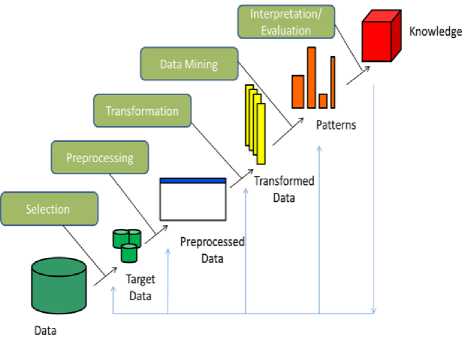
Fig.1. Knowledge Discovery Process in Data Mining [1].

As depicted in Fig. 1, the first step in data mining for discovering hidden patterns and extracting the knowledge is called as Extraction. Once the data is extracted the next step is to clean the data for processing. Cleansing of data is carried out to remove noise and undesirable feature. The process is called as ECTL (Extracting, Cleaning, Transforming and Loading). Handling static data is easier than dynamic data. The data nowadays have various forms like structured data (text data), unstructured data (audio, video, images). To transform this data to desirable properties different techniques are carried out like classification, clustering. The paper will discuss some of the data mining clustering techniques [12], [13].

• A.    Data Mining Algorithms

Data Mining follows three main steps in preparing the data for processing, reducing the data to concise it and extracting useful information. The major algorithms followed in data mining are classified into six classes [1]. The following steps are executed on raw data to obtain relevant information.

generalizes the known structure to new data. Such as Support vector machine, Multi-Layer Perceptron.

• B.    Data Mining Techniques

Various data mining techniques and systems are available to mine the data depending upon the knowledge to be acquired, depending upon the techniques and depending upon the databases [1].

• 1.    Based on techniques: Data mining techniques comprises of query-driven mining, knowledge mining, data-driven mining, statistical mining, pattern based mining, text mining and interactive data mining.

• 2.    Based on the database: Several databases are available that are used for mining the useful patterns, such as a spatial database, multimedia database, relational database, transactional database, and web database.

• 3.    Based on knowledge: Fig. 1 depicts the knowledge discovery process, including association rule mining, classification, clustering, and regression. Knowledge can be grouped into multilevel knowledge, primitive knowledge and general level knowledge.

• II.    Cluster Analysis

The simple means for analysing and managing large volume and complexity of data is to classify or group the data based on predefined categories or unlabelled clusters items. “Generally classification technique is either supervised or either it is unsupervised technique solely depending on whether they assign new items to one of a finite number of discrete supervised classes or unsupervised categories respectively [2], [7], [9], [10], while clustering is an unsupervised approach. The aim of clustering is to partition a finite unlabelled data set into a finite and discrete set of data structures that are hidden, rather than providing exact properties of unobserved samples generated from the same probability of distribution [2], [8], [9]. Clustering mainly follows two criteria for partitioning the unlabelled data items that include high similarity between the data objects within the same clusters and low similarity outside the clusters. Clustering leads to the formation of hard clusters.

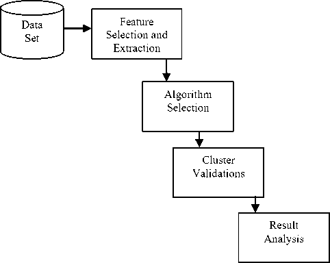
Fig.2. Steps for the formation of clusters and representing data inside clusters [2], [11].

It is important to learn the difference between classification and clustering. Both these terms can be explained by a simple example. Let a bucket contain some fruits say orange, grapes, apple and banana. Classification works on predefined knowledge or set of information. Classification algorithm will choose any feature like colour to be one of those features and will categorize the fruits depending on that set of information, while clustering has no such model for grouping the objects. Clustering defines its own model say shape to be one of those models. Clustering will group the above fruits based on shape. Clustering process can be carried out [2], [11].

• 1.    Feature Selection or Extraction: As referred in [2], [11] feature selection is the selection of relevant features from irrelevant features while feature extraction is the production of new features from predefined features.

• 2.    Selection and Designing of Clustering Algorithm: No such clustering algorithm is available which solves all the clustering problems. Different algorithms are available with different distance formula like Euclidean distance, Manhattan distance, Minkowski distance. It is important to first understand the problem carefully and then decide which algorithm is best suitable.

• 3.    Cluster Validation: Cluster validation is the assessment of the clusters formed. Testing of the clusters is done to make sure about the quality of the clusters so formed and guarantees that desirable clusters are achieved. Testing of the clusters can be done by three ways external indices, internal indices and relative indices [2],  [6]

• 4.    Result Analysis: The results so formed from the original set of the data is analysed to have an insight view of it and to ensure qualities of clusters formed are satisfied.

depending upon the type of clusters.

• III.    Partitioning Clustering Algorithm’S

Different initial points in clustering lead to different results [2], [14], [15]. Depending upon the properties of clusters formed clustering algorithms can be classified as Partitioning Algorithms, Hierarchical Algorithms and Density Based Algorithms [2], [15], [18].

• A.    Partitioning Algorithm

K-Means is the most famous and common type of clustering algorithm used to assign data objects to a cluster. Partitioning algorithm works by dividing the data objects into ‘k’ number of clusters partitions. Let dataset ‘D’, contains ‘n’ number of data items where ‘k’ is the number of partitions, partitioning algorithm assign ‘n’ number of data items to ‘k’ partitioners where (k ≤ n). These ‘k’ partitions are called as Clusters. The data items in a single cluster possess similar characteristics. The number of clusters formed should not be similar to each other as depicted in Fig. 3. Partitioning algorithms ensure that no cluster should be empty [17]. Partition algorithm does not follow any hierarchy like hierarchical algorithm follows, it divides the data objects in a single level. Partitioning works efficiently on a large dataset. A common criterion function for generating clustering output in partitioning algorithm is by using squared error algorithm [19].

E2 =Z^i^idl ^o)-y||)2 (1)

Where(II xi^-cj\\Y is a chosen Euclidean distance, while ‘cj ’ are the cluster centres, ‘ xi ^ ’represent the data objects.

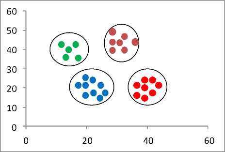
Fig.3. Objects partition in different clusters, where k=4 representing different data in the different cluster.

• B.    K-Means Clustering Algorithm

K-Means algorithm is the simplest algorithm which works on iterations to group the data objects in clusters [2]. Following the criteria of the sum of square error, K-Means algorithm has a time complexity of O (n). Trapping in local optima is the biggest problem with K-Means algorithm if the initial clusters are not chosen with care. K-Means algorithm aims at minimising the squared error. It is an unsupervised learning in which the ‘k’ is fixed apriori defines the initial cluster centre for every cluster the centroid should be defined careful and cunningly because the change in location also leads to change in results. The best way to place the cluster centres is to place them far from each other [16]. After the assignment of centres to the initial clusters, the next step is to associate each nearest points to a particular cluster. When all the data points are placed in the cluster recalculate a new centroid for the clusters. Repeat the process again until no data object changes its location. K-Means algorithm converges faster.

• C.    Algorithmic Steps for K-Means Algorithm

Let D= (d1, d2, d3,….,dn) be the data points in a dataset and S=(s1, s2, s3,....,sn) be the group of centres. The algorithm follows the below-mentioned steps for clustering [16]:

• 1.    Manually and randomly select the initial cluster centres ‘c’.

• 2.    Use Euclidean distance criterion function and calculate the distance between all the data points and the clusters centres.

• 3.    Information points with minimum distance from cluster centres are placed in that particular cluster.

• 4.    Above process is carried out for all the data points until all the points are placed in the clusters.

• 5.    Recalculate the new cluster focus ‘ci’ using equation mentioned below and again calculate the distance of every information point from new cluster centres.

• 6.    If no new reassignment of data points takes place then stop the process, if yes repeat the steps 2 and 3.

Si = (1/ci) l^di            (2)

Where, ‘ci’ is the number of data points in the ith cluster

• D.    Advantages of K-Means Algorithm

• 1.    K-Means is simple to implement and robust algorithm.

• 2.  K-Means Algorithm converges faster than any

• 3.  The algorithm can work efficiently on large

• 4.  Tighter and arbitrarily shapes of clusters are

• 5.  Compute faster than  Hierarchical clustering

other algorithm.

datasets and with a large number of attributes.

formed by K-Means clustering algorithm.

algorithm.

• E.    Disadvantages of K-Means Algorithm

• 1.    The algorithm cannot work on categorical data.

• 2.    Trapping into local optima is the biggest disadvantage of K-Means algorithm.

• 3.    Selection of initial clusters and its centroids are done manually and randomly which leads to variation in results if not done carefully.

• 4.    The Non-linear dataset cannot cooperate with K-Means algorithm.

• 5.    Numbers of initial clusters are fixed apriori.

• 6.    Noise and outliers affect K-Means algorithm.

• IV.    Hierarchical Clustering Algorithm’S

Instead of having a single partition like that in Partitioning algorithm, hierarchical algorithm forms a hierarchical structure of clusters called as a dendrogram. The tree like dendrogram can be split at different levels to produce different clustering of data. Hierarchical algorithm varies from Agglomerative clustering to Divisive clustering. In Agglomerative clustering algorithm, bottom-up approach is followed. This type of clustering assumes every document to be single clusters so as to group all the pairs of clusters in a single cluster that contains all the documents. Top down clustering proceeds by splitting the clusters recursively from a single cluster to multiple clusters. This approach is termed as divisive clustering algorithm [18].

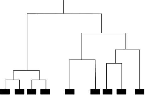
Fig.4. Representation of Hierarchical clustering using Dendrogram.

• A.    Algorithmic Steps for Hierarchical Agglomerative Clustering

  Given a set of ‘I’ data objects to be clustered and I*I matrix of distance based on similarity. S.C. Johnson in 1967 defined the hierarchical algorithm [27]:

• 1.    Initialization: Assign each object to a cluster in such a way that if you have ‘I’ objects than the number of clusters will be ‘I’. Each cluster is labelled by one object and the distance measures between the clusters are directly proportional to the distance between the objects they contain.

• 2.    Select a pair of clusters that have minimum distance (most similar) between them using single linkage metrics (similarity of most similar points) or complete linkage metrics (similarity of most dissimilar objects) and merge them in a single cluster. At this point, the numbers of clusters left are (I-1).

• 3.    Based on the distance (similarities), compute for each new cluster formed and previously formed clusters.

• 4.    Until all the clusters are not labelled in a single cluster of size ‘I’ repeat step 2 and 3. Once all data objects are placed in a single cluster of size ‘I’.

• B.    Algorithmic Steps for Divisive Clustering

Divisive clustering is further categorized into monothetic and polythetic. Monothetic clustering selects one attribute at a time to split the cluster while polythetic clustering employs all the attributes in a set of data to split the clusters. The Polythetic clustering algorithm is as defined below [20].

• 1.    Assign all the objects in a single cluster to reduce the clusters to a singleton cluster.

• 2.    Measure the distance between the objects based on any criterion and create corresponding distance matrix. The distance should be sorted in an ascending order. Also, choose a threshold distance.

• 3.    Select two objects that have the maximum distance between them that are most dissimilar to each other.

• 4.    If the distance between the two objects is less than the predefined threshold and no more splitting is possible then, stop the algorithm.

• 5.    Create new cluster from previous clusters.

• 6.    If a cluster is left with only one object stop the algorithm else repeat step 2.

• C.    CURE

Clustering Using Representative (CURE) is an Agglomerative clustering based method that works efficiently on large datasets and is robust to noise and outliers. CURE can easily identify the clusters of any shape and size. CURE intakes both partitioning clustering and hierarchical clustering which increases the scalability issues by sampling the data and partitioning the data. CURE is capable of creating ‘p’ partitions which enable fine clusters to be partitioned first. Secondly, CURE represents clusters by scattered points fixed apriori instead of a single centroid. CURE intakes numerical attributes. The consumption of memory for the selection of initial clusters is low in case of CURE [14], [20]. The algorithmic steps for CURE are [20].

• 1.    Collect a sample of the dataset.

• 2.    Split the sample into ‘p’ partitions of size ‘n’ to increase the speed of the algorithm by first performing clustering on each partition made.

• 3.    Label each data point to the partitions by using hierarchical clustering algorithm.

• 4.    Outliers are removed by first removing those clusters that are very slow in growing and later by removing clusters that are small in size.

• 5.    At the end label all the data to the sample. The processing is carried out in main memory so make sure to input representative point of the clusters only.

• 6.    Stop the algorithm after convergence is achieved.

• D.    CHAMELEON

An Agglomerative approach of hierarchical clustering makes use of linked graph corresponding to K-nearest neighbour. A graph is created in which each data points are linked to its K-nearest neighbour. Partition of the graph is carried out recursively to split it into small unconnected sub graphs. Each sub graph is treated as an individual sub–cluster and an agglomerative approach merges two similar clusters into one. To merge two subclusters interconnectivity and closeness of the clusters are taken into considerations. CHAMELEON is more efficient than CURE in finding arbitrary shapes of clusters [20], [21].

• 1.    Consider a data set D= (d1, d2, d3,…., dn) and ‘d1 to dn’ be the data points in a dataset.

• 2.    The dataset is to be partitioned to form clusters.

• 3.    Partition the dataset to form initial clusters using any graph partitioning approach.

• 4.    Merge the clusters to grow a big cluster by agglomerative technique taking into account interconnectivity and closeness.

• 5.    CHAMELEON is a feature driven approach.

• E.    BIRCH

• 1.    Construct a CF tree to load into memory.

• 2.    Set desirable range by constructing small CF tree.

• 3.  Sub-clusters to be re-clustered by using global

• 4.  Take the centroids of the clusters formed from

• 5.    Apply any existing algorithms to link data objects to its nearest seed to form a cluster.

• 6.    Stop algorithm.

clustering.

phase 3 as seed clusters.

• F.    Advantages of Hierarchical Clustering Algorithm

• 1.    The Hierarchical clustering algorithm is easy to implement.

• 2.    Multi- point partition of data objects takes place

• 3.    No pre-knowledge about the number of clusters is required.

• 4.    The Hierarchical algorithm is flexible regarding the level of granularity.

• G.    Disadvantages of Hierarchical Clustering Algorithm

• 1.    Difficult to handle noise and outliers

• 2.    Once the changes regarding merging or splitting of clusters are made then the algorithm is unable to undo those changes.

• 3.    In some case, dendrogram makes it difficult to correctly identify the number of clusters.

• 4.    Termination criterion of the algorithm is not definite.

• 5.    The algorithm turns out to be expensive in case of large datasets.

• V.    Density based Clustering Algorithm’S

DBSCAN (Density-Based Spatial Clustering of Applications with Noise) proposed by Martin Ester is a density based clustering algorithm which is capable of removing noise from spatial datasets and is efficient in finding arbitrary shapes of clusters [22]. It grows clusters depending upon the density of the objects present in its neighbourhood [23]. The implementation of partitioning the data objects are carried out by concepts like connectivity, density-reachable [14]. A point ‘p’ is said to be density-reachable from point ‘q’ is within ‘e’ distance of point ‘q’ and point ‘q’ also contain enough number of points within ‘e’ distance while ‘p’ and ‘q’ are considered as density connectivity if both ‘p’ and ‘q’ are within the ‘e’ distance and there exist a point ‘r’ which have enough number of points in its neighbour. A chain is formed in which each point corresponds to each other [24]. Both these concept depends upon epsilon neighbourhood ‘e’ that control the size of clusters and its neighbourhood and also on minpts.

• A.    Algorithmic Steps for Density-Based Clustering

Let D = (d1, d2, d3,…., dn) be the data points in a dataset. DBSCAN algorithm undertakes two parameters ‘e’ and minpts (minimum number of points corresponding to a cluster) to form a cluster [24].

• 1.    Initially, start from any random point that is not visited.

• 2.    Explore the neighbours of undertaken initial point by using ‘e’. The points nearby ‘e’ distance are the corresponding neighbours.

• 3.    If the initially random selected point has enough neighbouring points, then clustering process starts and all its corresponding neighbouring points are marked as visited otherwise the point will be considered as noise. Later this point can found in a cluster.

• 4.    If a point seems to be a part of the cluster, then its ‘e’ neighbourhood points are also the part of the cluster. Step 2 is repeated until all the points neighbouring to the initial point is placed in one cluster.

• 5.    A new point that is not visited is identified and the same process is repeated for the formation of further clusters or noise. Stop when all the points

are visited.

• B.    DENCLUE

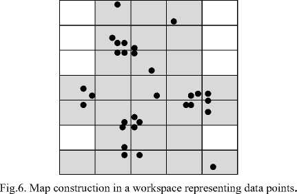
Clustering Based on Density Distribution Function (DENCLUE) is a clustering technique that is completely dependent on density function. The two ideas clinched by DENCLUE is that each data object’s influence can be described by using an influence function that describes the impact of data objects with its neighbours. Secondly, the overall density of data space is the summation of influence function of all the datasets. Cluster identification in DENCLUE is carried out by using density attractors where these attractors are the local maxima of influence functions. The computation of overall density in all the datasets is carried by forming a grid structure. DENCLUE is resistance to noise and insensitive to data ordering along with the feature of forming arbitrary shapes of clusters makes it unique but on the other side, it lacks in describing the clusters description properly. Thirdly, it is not a perfect choice for high dimensional datasets [20],  [21]. DENCLUE algorithms execute in two steps:

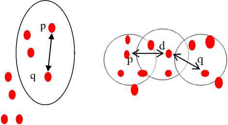
Fig.5. a) Representing Density-Connected between point’s ‘p’ and ‘q’ via ‘d’. b) Representing Directly Density Reachable from point ‘p’ to ‘q’.

• 1.    Pre-clustering phase: Map construction for the relevant and desirable workspace is constructed. The aim to construct the map for the relevant workspace is to boost the calculation for the density function to access the nearest neighbours.

• 2.    Clustering phase: In the final clustering phase, identification if density attractors are made and the related density attracted points are identified.

  

• C.    OPTICS

Ordering Points to Identify the Clustering Structure (OPTICS) is another clustering technique for forming clusters by using density function in spatial datasets. OPTICS follows the same path of DBSCAN but it converts one of the major limitation of density based clustering as its advantage ie. the problem of detecting meaningful and informative clusters from the data having varying density. In OPTICS clustering is carried out by placing the objects in such a way that objects that are close to each other become neighbours in the ordering. A dendrogram representation is structured that constitutes a special distance between each point containing the density of the points that is to be accepted by the clusters to allow both the points to belong to the same cluster [20].

• D.    Advantages of DBSCAN

• 1.    DBSCAN handles noise and outliers efficiently.

• 2.    The number of clusters is not specified in apriori like that in the case of K-Means algorithm.

• 3.    DBSCAN is capable of finding arbitrary shapes of clusters and can find clusters surrounding each other but are not connected.

• 4.    The parameters minpts and distance threshold can be set by an individual.

• E.    Disadvantages of DBSCAN

• 1.    Computation cost is high.

• 2.  DBSCAN intakes only two parameters and is

• 3.  Proper cluster description is not carried out by

• 4.    Not suitable for high dimensional datasets as the quality of clusters depends on distance measure and distance measure uses Euclidean distance which cannot render appropriate results with high dimensional datasets.

• 5.    DBSCAN lacks in handling clusters with varying densities.

highly sensitive to the parameters.

DBSCAN.

• VI.    Result Analysis

  WEKA is widely accepted in various domains like business and academia. WEKA project was aided by the New Zealand government [25]. In 1993, the University of Waikato in New Zealand began improvement of the initial WEKA (which came out as a combination of TCL/TK, C and Makefiles) [26]. Waikato Environment for Knowledge Analysis (WEKA) was envisioned to provide the researcher with a toolbox of learning algorithm along with a framework to implement new algorithms. WEKA being an open source environment is used for both machine learning and data mining. WEKA provides an analysis environment for various algorithms

like clustering, regression, classification and association rule mining. Attribute relation file format (.ARFF) or Comma separated value (CSV) format is opted by WEKA for information processing. In case the set containing information is not in the format we need to change it. WEKA allows users to interact with various graphical user interfaces like Explorer, Experimenter, Knowledge Flow and Simple CLI. The main interface is Explorer which constitutes various data mining tasks like pre-processing of the information set, classification, clustering, and association rule mining.

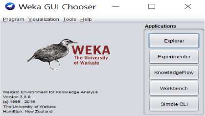
fig.7. view of weka tool.

The other main interface viz. experimenter is designed to perform an experimental comparison of the observational performance of algorithms based on many different evaluation parameters that are available in WEKA [25].

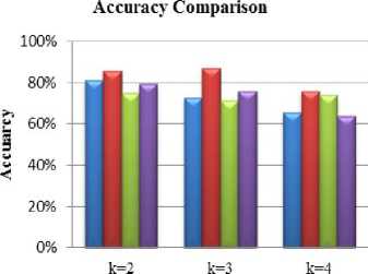
• A.    Results Analysis on Traffic Dataset

Table 1. Comparison Between Various Algorithms for the number of clusters k=2.

Number of clusters

■Density Based Clustering и Hierarchical Clustering

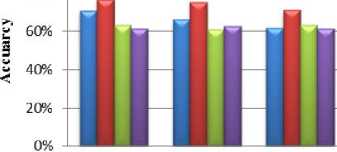
Fig.8. Accuracy comparison for traffic dataset.

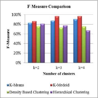
Fig.9. F-Measure comparison for traffic dataset.

^Density Based Clustering ■Hierarchical Clustering

Accuracy Comparison

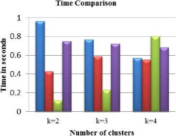
Fig.10. Time-comparison for traffic dataset.

• B.    Results Analysis on Ionosphere Dataset

100%

80%

k-2         k=3         k-1

^Density Based Clustering и Hierarchical Clustering

Fig.11. Accuracy comparison for Ionosphere dataset.

Table 4. Comparison between Various Algorithms for the number of clusters k=2.

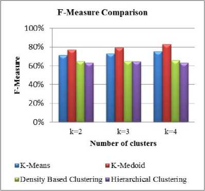
Fig.12. F-Measure comparison for Ionosphere dataset.

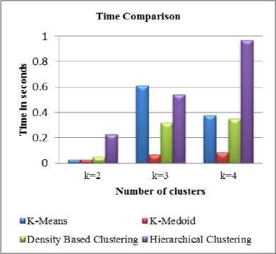
Fig.13. Time comparison for traffic dataset.

• VII.    Conclusion

Acknowledgment