Comparing the Performance of Naive Bayes And Decision Tree Classification Using R

Published Online December 2019 in MECS

Every industry is very concerned about data collection and requires accurate and appropriate information that will help it in decision making. This huge growth in data requires new techniques and automated tools that can be helpful in handling a vast amount of data by extracting useful information and knowledge from the transient data. Such a need for transformation leads us to a generation of a technique called data mining [1]. There are many algorithms that can be used to extract knowledge that can be useful in big data. But these algorithms differ in terms of how they “learn” about data for prediction at a high level. That is why the algorithms are classified into two categories: supervised learning and unsupervised learning. Supervised Learning is a learning method that is used to provide an algorithm with data which is already assigned with correct answer, that is some records will be tagged with the output variable of interest and then the machine will be provided with new dataset where the output variable will not be known and that the algorithm "learns" how to predict the output values for new records by analyzing the training data (portion of data used to fit a model) and using the labeled data [2]. Supervised learning is classified into two algorithms: classification and regression. Both are related to prediction.

• •    Classification algorithm:    A classification

algorithm takes discrete values and is used to predict the target class to which data samples belong. For example, given a dataset of images. On the basis of the training data we need to predict whether the image is of cats or of dogs and accordingly classify into class labels as "cats" and "dogs". The labels basically come in a categorical form.

• •    Regression Algorithm: A regression algorithm takes continuous values and is used to predict the real or continuous valued output. For example, we are given the size of the house, we need to predict the price (real output variable) for the house.

On the other hand, unsupervised learning is described as a learning method where only data is given without any outcome variable. Unlike supervised learning, there is no “learning” from datasets where outcome values are known. Algorithms are required to find the hidden structure from unlabeled data without any idea about the result to learn more about the data. The most popular and powerful machine learning tools used in classification and prediction are the decision tree and the Naive Bayes classification techniques. The algorithm for development of both the techniques requires training of data. The main focus of this paper is to compare the performance of both the Naive Bayes and decision tree.

Section I deals with the introductory part of data mining and also discuss about the types of learning and there classification. The related work is discussed in

Section II. In section III, we have given brief description about decision tree and what is used to build a decision tree. Section IV gives brief information about naive bayes. In section V, the implementation of both the classification techniques is explained along with the results and within this section, comparison of the result is also displayed followed by the advantages of both the techniques which are also discussed in sub sections B and C. The paper is finally concluded in section VI.

• II.    R elated W ork

A comparison between Naive Bayes and Decision Tree was performed by using weka software for data mining by Ahmad Ashari, Iman Paryudi, A Min Tjoa [17]. They took a training data set of 13 building parameters with each parameter has 4 possible values (4^13 data). They found that Naive Bayes is better classifier than decision tree and k-NN with the accuracy percentage 73.7% and the accuracy rate for decision tree was 58.9% and for K-NN, it was 56.7% which is much lower than Naive Bayes accuracy value. It was shown that in terms of precision Naive Bayes outperform the decision tree and k-NN when F-measure calculation is performed.

There is also study carried out by D. Xhemali, C. J. Hinde, and R. G. Stone [18] for the web classification by using Naive Bayes, Decision Tree and Neural Networks. The final results showed that Naive Bayes has higher accuracy than the other two classifiers. The accuracy of the Naive Bayes was 95.2% which higher than Decision Tree's accuracy rate which was 94.85%. In papers [20, 21, 22] Naive Bayes is also considered better than other classification techniques.

Another study was carried out by C. Anuradha1 and T. Velmurugan [24] that showed a performance comparison between Naive Bayes, KNN and JRip classifier using student performance dataset. They concluded that Naive Bayes performed well in comparison to other two classifiers. It had higher accuracy rate.

D.Sheela Jeyarani, G.Anushya, R.Raja Rajeswari, A.Petha lakshmi compared the performance of Naive Bayes and Decision tree using 10 datasets and obtained almost similar accuracy rate for both the classification techniques for most of the datasets. Their study suggested for the development of hybrid algorithms, that combines Decision Tree and Naive Bayes with different optimization techniques.

A study by S Rahmadani, A. Dongoran, M. Zarlis and Zakarias performed feature selection by using Genetic Algorithm and took three datasets for comparison: Iris dataset, Glass dataset and Germany Credit dataset. They concluded that decision tree performed slightly better than Naive Bayes. This only occurred for feature selection by using Genetic Algorithm and also suggested Genetic algorithm can be useful in improving the accuracy of both Naive Bayes and Decision Tree. But Decision Tree performed better than Naive Bayes because of optimization technique.

• III.    D ecision T ree

A decision tree is a tree structure that is considered as one of the popular tools for classification and prediction which includes a root node, an internal node, and a leaf node. Each internal node of the tree corresponds to a test on an attribute, each branch represents a decision (rule), and each leaf node (terminal node) corresponds to a class label (categorical or continuous value). A decision tree is drawn upside down with its root at the top of the tree and leaf node at the bottom of the tree representing the outcome variable.

The tree grows by splitting the training set into two or more categories (sub-nodes or subsets) which are also called decision nodes. Each subset is made in such a way that each of them should contain data with the same value for an attribute [3]. Continue the splitting on each derived subset in a recursive manner called recursive partitioning until the leaf node is found on each branch of the tree. The major challenge is the identification of the root node in the decision tree for each level and such problem is known as attribute selection. Thus, there are different decision tree algorithms that use different measures to split the nodes on all given values and then select the efficient split that result in most homogeneous sub-nodes, in other words, attributes are selected on the basis of purity (belonging to a single class) with respect to target variable [4,5]. The two most popular attribute selection and purity measures are Gini index and entropy which is used in the Information Gain.

• A. Calculation of Purity and Attribute Selection

Before the construction of a tree, the most important step is the attribute selection and measure of purity which can be done by using:

• 1)    Gini Index

• 2)    Entropy and Information Gain

• 1)    Gini Index

Gini Index is a metric that is used to measure inequality among chosen random variables and can be defined as

I (A) =1-∑™=1 ^к             (1)

Here, m classes denoted by k=1, 2….m. Р^

=proportion of observation that belongs to class k. This equation takes the value between 0 (if all observation belongs to the same class) and (m-1)/m (when m classes are equally represented). That is, a lower Gini index of any attribute should be preferred among other attributes . CART (Classification and regression tree) algorithm uses the Gini index for attribute selection for the construction of decision tree.

• 2)    Entropy and Information Gain

ENTROPY: Another method for testing the purity of any attribute or sub-node and perform attribute selection for the root node is by using entropy and information gain. Entropy is the measure of uncertainty in the information that is being processed which is defined as

Entropy (A) = -∑ _k^P_klog₂ ( P_k )         (2)

For log function use log(x, 2) and. p =proportion of observation that belong to class k. Its value also falls between 0(most pure, that is all attributes are homogeneous and belongs to one class) and log2 (m) [5]. The entropy value for a class attribute can also be calculated by using the formula:

Entropy= - -^—log₂ (—)- -^—log₂ (—)   (3)

P+N \P+N/ P+N ^3 ^y

It is important to note that lower the entropy, higher are the chances of an attribute to be selected as the decision node of the tree.

INFORMATION GAIN : The next method is to calculate the information gain for each attribute of the dataset. Information Gain is based on the decrease in the entropy value when a node is used for data set partitioning that result in small sub-nodes. The information gain formula is given.

For each attribute, Information gain can be calculated as

Information Index (Pi, Ni) = p 1     / pA N 1 Z N _ч

- --- log₂ (   )---- log₂ (   )       (4)

P+N \P+N/ P+N      ^3 ^^ ^y

For this formula, we need to apply another formula for entropy for attributes i which is defined as

Entropy (attribute) = ^∑ Pi+Ni (Information Index (Pi, Ni))

As shown above, the entropy value for a class attribute can also be calculated by using the formula given in equation 3 (from (3)).

Here in the above equations, P= Possibility of positive or ‘yes’ value for an attribute and N=Possibility of negative or ‘no' value for an attribute. In this, it is required to calculate the entropy of each value of a single attribute and combine the resulting entropy of the values to get the entropy for the single attribute in the dataset. After this step, we are required to find the gain value for an attribute that will decide which attribute will be taken as a decision node. Higher the gain value, higher the chances of becoming a decision node.

The gain formula can be written as

Gain= Entropy (class) - Entropy (attribute)      (6)

Information gain uses the entropy only to get information about which attribute will best suit for the split in the dataset.

Various decision tree algorithms can be used for the construction of a tree by using the data set and by measuring the purity of the attributes like CART, C4.5,

SLIQ, Random forest etc. The ID3 algorithm uses the Information gain and entropy for the feature selection and for the calculation of purity of the attributes. For the implementation of the tree, we can use the caret package, data.tree package that is basically used for the selection of best feature and optimize the code of decision tree.

Whereas the CART algorithm uses a metric named Gini Index for the attribute selection for the decision tree. The CART algorithm can be implemented using the rpart package which is used for the recursive partitioning and regression and classification trees, that is, CART can handle both classification and regression trees.

• IV.    N aive B ayes C lassification

In mathematical theory, we calculate the probability of occurrence of an event only for a single event. We even calculate the occurrence of group events that occur together. But, in data science, we use the knowledge of probability to calculate the proportion of where the second event will occur. That is why the Naive Bayes classification is introduced which can predict the outcome by using the training dataset. But before understanding the concept of Naive Bayes it is required to first understand the concept of Bayes algorithm as Naive Bayes is based on the formula of Bayes theorem.

• A.    Bayes Theorem

In machine learning, Bayes theorem provides a way to calculate the probability of a prior event (meaning an event is occurring), given that another subsequent event has occurred. Bayes theorem is a method that is used for predicting values, that is, it gives us a formula for computing the probability that a certain record belongs to a given class, given with record’s attribute [7]. It only makes the prediction on the basis of prior knowledge (meaning, probably guess on an outcome without any information about its attribute) [8]. But with the addition of more evidence, the prediction made by the theorem also changes which is important for the theorem for classification [9]. The main formula of the Bayes theorem is given as:

P (A|B) =

p ( в | A ) P ( A ) P ( В )

Here, A and B are events where B is evidence and according to this equation, we are calculating the probability of the event A given that B is true. By the word evidence, we mean an attribute value of an unknown instance [8].

P (A) is the prior probability (probability of an event without any evidence is seen) and P (A|B) is the posterior probability (probability when evidence is seen) and P (B|A) is said as the conditional probability of B given A [8]. Our main concern is to calculate the posterior probability of P (A|B).

• B.    Naive Bayes Classification

The Naive Bayes classifier is one of the most simple still more sophisticated techniques of classification which combine the set of given predictors information into the naive rule in order to get an accurate result of classification [10]. That is, the probability of a variable belonging to a class can be obtained not only by using the prevalence of that class but also on the basis of additional knowledge on that data. This method has a set of supervised learning algorithms that are based on Bayes’ Theorem with an assumption of independence among predictors. It means that the features in a class are independent of any other features. So we divide the evidence into different independent attributes. This independent feature assumption is not always correct but sometimes works fine in practice [12]. That is why this classifier is called Naive Bayes classifier. Naive Bayes classifier can be used for both continuous and categorical variables. It is based on the Bayes formula that is the probability of event A given B evidence which is given above also as [11]:

P (A, B) =P (A) P (B)            (8)

Through this formula and using the concept of Bayes theorem (from (7)) the final formula is as follows:

P (A|B)

_Р (В1А)Р(А) Р(В)

Here, A is a class and B is an instance. A represents the dependent event which means a predicted variable and B represents the prior event which means a predictor attribute. This Bayes formula is already explained above in (1). Now the final step of the Naive Bayes algorithm is to find the maximum probability [14]

y = ar дтаХуР (у)П?= 1 ^(^|у) (9)

That is, it is required to classify the data to the class that holds the highest probability value.

• V.    I mplementation and R esult

In this paper, RStudio is used to perform the implementation of the classification of a decision tree and Naive Bayes using R language because RStudio is one of the most famous and easy to use tool which makes the task of construction of any structure more flexible than other tools.

In the below example, the decision tree is implemented by using the rpart package. And for the Naive Bayes, the implementation part is performed by using e1071 and caret. The dataset used for the comparison is based on the class of student’s marks along with 16 attributes. This dataset is used to predict the student’s performance on the basis of available features. The features in this dataset are divided into three main categories [14, 15]:

• 1)    Demographic features which include gender and nationality, place of birth features.

• 2)    Academic features which include educational stage, grade level, and section ID, a topic which subject the student is learning from the school in the class, semester.

• 3)    Behavioral features like a raised hand in class, visited resources, group discussion participation, parent answering the survey and school satisfaction, student absence days.

For the classification purpose the class used in this dataset is based on total grade of a student, that is, the students are classified on the basis of three levels: L (for low grade between 0 and 69), M (for middle level grade values from 70 to 89), H (for high level grade values from 90 to 100). Based on the learning of the machine, the test dataset is being predicted. One most important thing is that there are different types of decision. A continuous quantitative data is used in the regression tree that is if we are using the information to predict a number it will be a regression tree whereas a qualitative data (category) is used in classification tree.

The basic idea for the classification tree is to take a single dataset of any size which will be a training data set. This is used to train the model that will be used for the prediction of class for unlabelled features and testing the accuracy of the model using test dataset. Now for the given dataset, we need to first build the model that will be needed to classify our test dataset, that is, at which level of the grade a student belongs to according to the features of a student in the dataset.

We have first checked the data by writing, str (data1). After this command, we concluded that the target indicator or class here is the Class column which specifies the grades on three levels for the evaluation of student’s performance in the school. We have 480 observations with 17 columns in which 16 are the variables or attributes and 1 column is of class. We have our data into training and test data set. It is necessary because with the training dataset we need to train our algorithm about the structure and only then we can use the test dataset to check the accuracy and prediction of our model. We can also create different datasets without dividing the dataset into two datasets.

First, to perform this we need to include rpart library and rpart.plot library which is used to specify the model data, formula, and parameters for decision tree. The main things followed in the creation of decision tree includes construction of tree using training dataset, perform prediction for test dataset and calculating accuracy to check model performance, and the last step is pruning to optimize the tree to get an accurate result and again calculating the accuracy of the tree.

Now, for the creation of a tree, we will use rpart() for the growth of the tree. The rpart can run a regression tree if the response variable or class is numeric otherwise it will perform an operation according to the classification tree if the response variable is a factor or categorical value. When we are using rpart, by default it uses Gini index to perform splitting operation when performing classification of the tree but we can use information gain for splitting by using split='information' in the parms parameter.

Student<- rpart(Class~.,data = train,parms = list (split = 'information'), method = "class",minsplit = 2,minbucket=1)

In this code, the method ='class' is written which is used only for classification tree and anova is used for the regression tree. Now we will perform prediction as it is necessary to cross-check the validity of our model with our test dataset where the outcome is not known. The function predict () is used to predict the test data class according to the learned decision tree using rpart. By using the below function, we can predict the class level for students in the test dataset and can test how well the model is performing by learning from the training dataset. We also need to evaluate the accuracy of this model.

pred<-predict(Student,test,type=c("class"))

print(pred)

accuracy<-sum(test$Class==pred)/length(pred) print("The accuracy before pruning") print(accuracy*100)

The accuracy before pruning is 70%

Levels: H L M print(“The accuracy before pruning)

"The accuracy before pruning"

print(accuracy * 100)

The output of values after executing the printcp() function for the display of the cp value along with xerror is given in Table 1. below:

Table 1. The output of printcp () execution after the accuracy calculation

Sno	Cost-complexity pruning	nsplit	Rel error	Cross-validation error	xstd
1	0.209184	0	1.00000	1.00000	0.046485
2	0.204082	1	0.79082	0.95918	0.046774
3	0.122449	2	0.58673	0.58673	0.44509
4	0.015306	3	0.46429	0.52041	0.043111
5	0.012755	5	0.43367	0.51531	0.042990
6	0.011905	7	0.40816	0.52041	0.043111
7	0.010204	14	0.29082	0.51531	0.043231
8	0.0100000	20	0.22959	0.52551	0.43231

Pruning : It is said that the bigger tree gives high accuracy but it can also lead to over-fitting. Over-fitting means that the model works well and gives an excellent result for the training data but fails to work correctly with the test data because of an increased feature of the training dataset. Thus, optimization of the tree size is required to improve the level of accuracy and prediction method. The solution for the over-fitting is to minimize or stop the growth of the tree. This can be done by using the pruning technique which is used in determining the size of the decision tree. To perform pruning it is necessary to remove the cross-validation error and we should select the cp value which is used for pruning the tree for higher accuracy to avoid over-fitting of the data.

The best step to prune a decision is by using the complexity parameter of the smallest tree with the smallest xerror. From figure 4, we can see that the best value for cp is 0.01 that has xerror 0.51531. So we will use cp slightly greater than 0.01 values which are 0.02 for pruning the tree. Now, the pruning function is implemented as cpp<-

pfit<-rpart(target,data=train,parms = list(split = 'information'),method="class",control               = rpart.control(cp =0.02)

Finally, the tree is pruned which is displayed in figure 5 and the accuracy is calculated after the pruning process and the confusion matrix is also obtained which are as follows:

Fig.1. Flowchart of Decision tree after pruning and than calculating the accuracy after pruning.

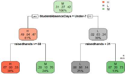
We can see that the split is performed on the attributes raisehands< 31 and raisedhands>= 58 with the root node StudentAbsenceDays=Under7. The confusion matrix of the decision tree is given as:

confusion Matrix and statistics

Actual Prediction н l м

H 25 1 20 L 0 25 11

M 12 10 36 overall statistics

H   L   M

0.2647059 0.2911765 0.4441176

Conditional probabilities: gender

Y    F   M

H 0.5217391 0.4782609

L 0.1287129 0.8712871

M 0.4117647 0.5882353

Accuracy 95% CI No information Rate P-value [Acc > NIR]

Kappa :

Mcnemar's Test P-value :

0.6143

(0.5284, 0.6953)

0.4786

0.0008569

0.4055

0.3843414

StudentAbsenceDays

Y Above-7 Under-7

H 0.05434783 0.94565217

L 0.88118812 0.11881188

M 0.31372549 0.68627451

Fig.2. Confusion matrix output of the decision tree for classifying student performance

The accuracy value for the final tree is given below after pruning is:

> print ("Accuracy after pruning") "Accuracy after pruning"

> print (accuracy*100)

61.42857

The final accuracy rate of the model is 61.42%. This shows that the model slightly improved after pruning and we get the final decision tree for the given dataset. Now, the calculation of accuracy for Naive Bayes will be performed and the comparison will be done to find out which classification technique is better for classification.

• A.    Naive Bayes Classification Using R

  For Naive Bayes implementation, e1071 and caret are used. The e1071 package is used to provide functions of probability, for class analysis, naiveBayes () function that makes the calculation for Naive Bayes classifier easy. This package made the task for classification using Naive Bayes much more simple [16]. The two important steps in Naive Bayes include the use of naiveBayes () function and after that prediction is performed to test the performance of the model along with accuracy calculation. The division of training dataset and test dataset is already performed in the above part. Now next step of Naive Bayes classification is to use naive Bayes() function which is included after the e1071 library is included. The code along with the output is as follows:

model= naive Bayes(Class~.,data=train,laplace=1) >model

Naive Bayes Classifier for Discrete Predictors

Call:

A-priori probabilities:

Y

>class(model)

• [1]    "naiveBayes"

>model$apriori Y

H L M

90 99 151

To create the Naive Bayes model, we applied the Naive Bayes function along with the Laplace parameter. The Laplace is initialized with 1 as Naive Bayes is based on the calculation of conditional probabilities of each feature on each class. It is found that if any feature has zero probability of occurrence for a class then it can lead to posterior probability to be zero for that class. To avoid this, Laplace=1 is included in the above code. With the use of model$apriori we represented the class distribution in the data set, that is, the prior distribution of the classes is represented here. As we can see there are 90 belongs to “H” class, 99 belongs to “L” class and 151 belongs to the "M" class of the training dataset. And the a-prior probabilities that are obtained from naive Bayes () function are the prior probability. Now it is required to perform the prediction function for the test dataset. The density plot for the original dataset, training and test dataset of the student's performance classification is shown below:

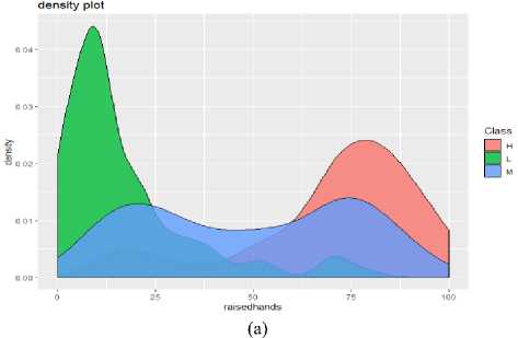
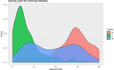
(b)

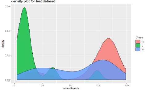
(c)

Fig.3. Density Plot for the (a) original dataset of student’s performance classification, (b) training dataset, (c) test dataset for the student’s performance classification

Prediction : In the above part, the naive Bayes () function is used which return the object of the class which is displayed by class (model) and gets "naive Bayes". Such an object is used for the prediction function which can predict the outcome for unlabelled variables. It returns an object of class "naive Bayes". Now we can perform prediction using the predict function that uses the model for classification of observations on the basis of conditional probability that is obtained in the above code. The predict function is implemented along with the confusion matrix and accuracy calculations as output are as follows:

pred<-predict(model,test,type="class")

table(pred)

table(test$Class)

cmatrix<- table(pred,test$Class,dnn=c("Prediction","Actual")) cfm<-confusionMatrix(cmatrix)

>cfm

Confusion Matrix and Statistics

Actual

Prediction H L M

H 43 0 9

L 2 22 4

M 35 1 24

Overall Statistics

Accuracy: 0.6357

95% CI: (0.5502, 0.7153)

No Information Rate: 0.5714

P-Value [Acc> NIR]: 0.0725235

Kappa: 0.4323

Mcnemar's Test P-Value: 0.0002529

• > Accuracy

[1] "63.57%"

Here, the table function stores the information regarding conditional attribute and class. The result of the table function is stored in the cmatrix variable which is passed in the confusionmatrix () function to display the actual and predicted values in the confusion matrix for determining how accurately the model is performing classification task. From the above output, the accuracy percentage of the Naive Bayes classification for classifying student’s performance is 63.57%.

• B.    Result

Table 2. Result of accuracy of classifiers

Dataset used: Students performance	Naive Bayes Classification	Decision Tree
Accuracy	63.57%	61.42%
Kappa value	0.4323	0.4055
Mcnemar’s Test P-value	0.0002529	0.383414

From the above sections and from Table 2., it is clear that Naive Bayes has better accuracy percentage which is 63.57% than decision tree classification whose accuracy rate is 61.42%. The accuracy can further be improved further in the future. As mentioned in the table, the kappa value is used as a statistic to determine how closely the values are classified by the classifiers. It is used to evaluate the classifiers amongst themselves. According to Landis and Koch, the kappa value 0.4323 comes under the category of moderate and 0.4055 comes under the category of fair [23]. There are also other studies that get Naive Bayes accuracy much better than the decision tree's accuracy.

• B.    Advantages of Decision Tree

• •    Easy to develop the resulting model. The model can handle any type of data whether the calculation has qualitative or quantitative values.[19]

• •    Decision tree is non-parametric. So there is no compulsion for independent variables to follow any kind of probability distributions.

• •   Decision tree eases the process of accurate

predictions for different types of application.

• •   By using information gain or Gini index it can

measure the priority of each variable in the training data set.

• •    Through Decision tree, visualization of results can be done which further helps in decision making.

• C.    Advantages of Naive Bayes

• •    The Naive Bayes classifier is easy, fast, to implement and can handle large datasets in comparison to other classification techniques.

• •    The Naive Bayes can work on both binary and multi-class classification problems and can handle continuous and discrete datasets.

• •    Though Naive Bayes relies on the conditional independence assumption, but even if this independence does not hold, it will still perform better and will give results.

• •    The Naive Bayes classifier is not sensitive to unrelated features.

• VI.    C onclusions

This paper gives a brief description of the decision tree and the Naive Bayes classification. It explains the concepts that are necessary for the development of a decision tree and Naive Bayes. It also gives a little information about the two most popular algorithms ID3 and CART algorithm which are used for the implementation of a decision tree. In this paper, how a decision tree and naive can be built is explained through an experiment by taking a student's performance classification dataset and the concept of both the classification techniques are implemented in RStudio using R language. The basic steps that are always important for the development of a decision tree are: first take two data set (training and test dataset) and build the tree based on training dataset so that the machine can "learn". The second step is to check the prediction of tree using test dataset. The third step is to check the accuracy of the tree to remove cross-validation error. In the example, we have focused on all these steps to give an optimized decision tree. Also, the steps that are important for Naive Bayes are explained. The concept of Bayes theorem is also briefed in the paper. Finally, accuracy is calculated for both the classification techniques and it is found in the experiment that Naive Bayes performed better than the decision tree. Hence, the Naive Bayes algorithm gives a significant improvement over the decision tree algorithm.

Our study as exhibited in this paper concludes that Naive Bayes classifier is a simple algorithm that gives more accurate output. The Naive Bayes algorithm performs better than Decision Trees when applied to large data sets.

• VII.    F uture S cope

  The conclusion drawn from this study will be applied to classify our Mobile Network Preference data set that we have collected from 1000 users.

A cknowledgment

I would like to express my special thanks to my teacher Dr. Reema Thareja for her valuable support, her patient guidance and for giving me this golden opportunity to work on this research work with her.