Comparison of Predicting Student’s Performance using Machine Learning Algorithms

Published Online December 2019 in MECS

To foresee how students may perform amidst their learning procedure is a stunning errand paying little appreciation to constant addition of data in the databases identifying with students scholastics in establishments of higher learning. As shown by [1], the academic organization frameworks are not composed genuinely to help illuminating executives with looking at which students are in hazard of dropping out of school or college. An educational framework has expansive measure of enlightening information. This information might be students' information, instructors' information, graduated class information, resource data, and so on. Educational data mining is utilized to discover the models in this data decision-making. There are two sorts of Educational structure: Traditional Education structure and Web based learning framework. For higher instructive foundations whose objective is to add to the enhancement of nature of cutting edge training, the achievement of generation of human capital is the subject of a consistent investigation.

Thusly, the craving for students' prosperity is critical for advanced education organizations, in light of the manner in which that planning procedure is the capacity to address students' issues.

Data Mining (DM) is the way toward finding fascinating examples and learning from a lot of information [2]. Educational Data Mining (EDM) is the utilization of Data Mining structures on informational data. The goal of EDM is to separate such information and to choose educational research issues. EDM directs growing new techniques to inquire about the educational data, and utilizing Data Mining frameworks to even more immediately handle student learning condition [3, 4]. The EDM framework changes over characteristic information beginning from instructive structures into essential data that could massively impact educational research and practice. Educational Data Mining experts consider a game plan of territories, including individual learning from educational programming, reinforced system learning, PC adaptable testing, and the segments that are associated with student disillusionment or non-support in courses [5, 6]. Educational data mining utilizes different strategies, for example, Decision Trees, Neural Networks, Naïve Bayes, K-Nearest neighbor and various others. Prediction and examination of student execution is a fundamental point of view in informative condition. Student's educational execution is an essential factor in building their future. Scholarly execution of learner isn't a consequence of only a solitary picking feature other than it energetically relies upon various parts like personal, socio-economic, psychological and other environmental variables.

The rest of this paper is composed as pursues: Section II provides a review of the machine learning algorithms utilized in this study. Section III gives data collection process and some insights to the structure of data and experimental matrices. Section IV shows the results and discussions, and Section V concludes the study.

• II.    Related Works

We surveyed many papers which are utilized machine learning algorithms for predicting the student performances such as Decision Tree [J48, CHAID (CHi- squared Automatic Interaction Detector), REPTree (Reduced Error Pruning Tree), Simple cart, ID3 (Iterative Dichotomiser 3), C4.5, CART (Classification and Regression Tree), and NBTree (Naive Bayes Tree)],

Random Forest, Support Vector Machine, Naïve Bayes, K-Nearest Neighbor, Multilayer Perceptron, Sequential Minimal Optimization, and Deep Neural Network. These details are depicted in table 1.

Table 1. Literature survey

S. No.	Algorithm	References
1	Decision Tree (DT)	[7-28]
2	Random Forest (RF)	[22]
3	Support Vector Machine (SVM)	[23][29]
4	Naïve Bayes (NB)	[7][13,14][18][29]
5	K-Nearest Neighbor (KNN)	[14][23]
6	Deep Neural Network (DNN)	[29, 30]
7	Multilayer Perceptron (MLP)	[7] [13] [17,18] [20] [29]
8	Sequential Minimal Optimization (SMO)	[7][14][18]

Kaur et al. [7] focused on identifying the slow learners by creating predictive model using classification algorithms. Real world data were taken and tested in WEKA tool using Naïve Bayes, J48, REPTree, SMO, and Multilayer Perception. Among all classifiers Multi Layer Perception performs best with 75% accuracy. Lakshmi et al. [8] analyzed the performance of decision tree algorithms such as ID3, C4.5 and CART on student’s data. The accuracy of CART was higher when compared to others. Ogwoka et al. [9] created the model for predict academic performance of students using combination of K-Means and Decision tree algorithm to reduce drop rate and improve the performance of students. Kabra et al. [10] used Decision tree algorithms on engineering students’ history of performance data to generate the model which is used to predict the students’ performance. Anupama Kumar et al. [11] applied C4.5 on student’s internal assessment data to predict their performance in the final exam that are to pass or fail. Josip et al. [12] developed a model using decision trees for predicting the academic success of students. Data collected from Faculty of Economics and University of Osijek and tested on REPTree algorithm that produced 79% as the highest rate of classification.

Edin Osmanbegović et al. [13] applied MLP, J48 and NB to predict the academic success of students. They collected from University of Tuzla and the Naïve Bayes outperforms with 76.65% accuracy. Livieris et al. [14] developed hybrid predicting system using six algorithms in WEKA tool with 2 different dataset for first and second semesters. 3NN for first and BP for second semester dataset produced better accuracy. Kolo David Kolo et al. [15] predicted academic performance of the students using IBM (SPSS) and CHAID. Mashael et al. [16] used EDM to predict students' final GPA according to their grades in earlier courses. They collected data from King Saud University and applied the J48 in WEKA tool. Jai Ruby et al. [17] predicted the performance of Students in Higher Education using classification algorithms like REPTree, ID3, Decision Table, J48, Bayesnet, MLP, BFTree, Simplecart and NBTree. MLP produced 74.8% high result in WEKA tool.

Ramesh et al. [18] identified the factors that influencing the performance of students in final assessment and predicted the grade of students using Naive Bayes, MLP, SMO, J48, REPTree algorithms in WEKA tool. MLP produced 72.38% accuracy which is higher than others. Pratiyush Guleria [19] used J48 decision tree algorithm in WEKA tool and calculated the Entropy of the attributes and taken Information Gain as the root node. Pimpa Cheewaprakobkit [20] predicted Student Academic Achievement using Decision Tree, Neural Network in WEKA tool with the dataset data set comprised of 1,600 records with 22 variables. Decision tree was outperformed with 85.188% as accuracy. Bashir Khan et al. [21] predicted the final grade of students using J48 Decision tree algorithm.

Shaymaa E. Sorour et al. [22] built an interpretable model using DT and RF. They applied comment data mining technique to predict grade and extract rules. Buniyamin et al. [23] predicted and classified student’s academic achievement based on CGPA using Neuro-Fuzzy. Quadriet et al. [24] predicted the drop out feature of students based on CGPA using J48. Christian et al. [25] identified the factors affecting the students’ performance. They considered students’ education, personal, admission and academic data using NBTree algorithm. Muslihah Wook et al. [26] predicted students academic performance then compared with ANN (Artificial Neural Network) and (clustering and decision tree) classification techniques. Shaleenaet et al. [27] used an effective method to identify and predict the dropout students using decision tree classifiers and discussed about the class imbalance problem.

Mrinal Pandey et al. [28] constructed the decision tree model by considering some significant factors using algorithms J48, NBtree, Reptree and Simple cart in WEKA tool. Bo Guo et al. [29] developed a classification model to predict student performance using Deep Learning. They used NaiveBayes, MLP and SVM and result were compared with SPPN (Students Performance Prediction Network) which provides high accuracy. Bendangnuksung and Prabu [30] used deep neural network in python with keras library for prediction of student performance.

• III.    Implementation

We have used six machine learning algorithms to prediction of student performances in R Programming on

Kaggle dataset and these results are compared.

• A.    Dataset

The wellspring of information for building the proposed deep neural system to predict the students' performance         is         acquired         from It is an instructive dataset gathered from learning the board framework called kalboard 360. The informational collection stretches out into 500 students with 16 features. The features are grouped into three primary classes: Demographic features such as gender and nationality, Academic background features such as educational Stage, grade Level and section and Behavioral features, such as raised hand on class, visited resources, parent Answering Survey and Parent School Satisfaction. The dataset details such as Name of the features, category, data type, number of values and description are in table 2.

Table 2. Data set

Features Category	Name of the attributes	No of Values	Description
Demographical Features	Gender	2	Female or male
	Nationality	14	Nationality of student
	PlaceofBirth	14	Place of birth for the student
	ParentResponsible	2	Father or mum
Academic Background Features	Stages	3	Primary, middle and high school levels
	Grades	12	Grade of the student
	SectionID	3	A, B, C
	Topic	12	Course topic
	StudentAbsentday	2	Above-7, Under-7
	Semester	2	First or second
Behavioral Features	Raisedhand	0-100	Student Behavior during interaction with e-learning system
	VisitedResource	0-100
	Viewing Announcement	0-100
	Discussion Group	0-100
Parents Participation on learning	ParentAnswering	2	Yes, No
	ParentSatisfaction	2	Good, bad

The 16 features are independent variables and the class is dependent variable with three classes such as low, middle and high. Among 480 records the target variable Class contains three values such as 1 as high (142 instances), 2 as medium (211 instances) and 3 as low (127 instances) and shown in fig. 1.

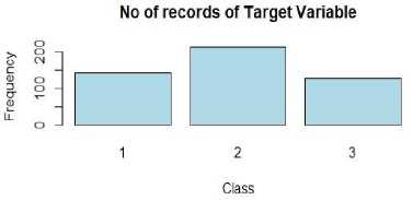
Fig.1. Histogram of target variable with 3 classes.

• B.    Evaluation metrics

We used many matrices to calculate the performances of the six machine learning algorithms. These are confusion matrix, True Positive Rate, True Negative Rate, Accuracy, Precision, Recall and F-Score.

• •    TP (True Positives) – TRUE, TRUE

• •    TN (True Negative) – FALSE, FALSE

• •    FP (False Positive) – TRUE, FALSE

• •    FN (False Negative) - FALSE, TRUE

Confusion matrix is known as the plot of the classification of the NxN matrix. It is in table 3.

Table 3. Confusion matrix

	Predicted
Actual	T	F
T	TP	FN
F	FP	TN

Equation (1) – (6) indicates the matrices such as TPR, TNR, Accuracy, Precision, Recall and F-Score. TPR (True Positive Rate) is a measure of proportion of what numbers of true positives were distinguished out of all the number of positives identified. It is also known as sensitivity.

TP TP

TPR = — = _!_!__             (1)

P TP+FN                 v '

TNR (True Negative Rate) is the proportion of true negatives and complete number of negatives we have anticipated. It is also known as specificity.

TN TN

TN R = — = ——          (2)

N TN+FP                 v '

Accuracy is the measure of how great is our model. It is relied upon to be more like 1, if performance of our model is admirably.

F =2.

precision . recall precision+recall

TP+TN _ TP+TN

P+N TP+TN+FP++FN

Precision is characterized as how many chosen items are significant. That is, how many of the predicted values are actually correctly predicted.

Precision =(4)

TP+FP

In the event that precision is more like one, we are progressively precise in our expectations. Recall shows that how many relevant items were chosen.

Recall =(5)

TP+FN

F-score is the measure of accuracy. In fact, it is the consonant mean of precision and recall.

• IV.    Results and Discussions

The main goal is to predict the performance of the student based on the various input variables which are retained in the model. The classification model was built using several machine learning algorithms and their results are compared. Needed packages are installed and loaded for different machine learning algorithms. The R Programming is used. Each classifier is applied for testing options - cross validation and data size is 480 that is divided into 70% as training data (337 instances) and 30% as testing data (143 instances) for the implementation of all the algorithms. The plot of the overall data is clearly shown in Fig.2.

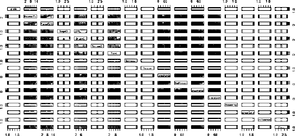
Fig.2. Plot of the overall data.

• A.    Naïve Bayes

Naïve Bayes is a classification Technique based on the Bayes’ Theorem. Thomas Bayes proposed this Theorem. This model is simple to build and mostly used for extremely large data sets [13].

The naivebayes library is installed. Loaded the data with read.csv() method. Converted the target variable as factor using as.factor() method. Created the training and testing data. Applied naïve bayes in training data using naïve_bayes() method. Mean and standard deviations are displayed for all attributes with 3 classes. Plotted the method for all the 16 attributes except target attribute (class) and the plot of the attribute StudentAbsenceDays is displayed in fig. 3. Color lines indicate the classes like Red for class 1, green for class 2 and blue for class 3.

Equation (7) and (8) are used to predict the loss as 27% and the accuracy as 73% respectively from the testing data in Naive Bayes algorithm.

1- sum ( diug ( tab ))/ sum ( tab )       (7)

sum ( dicig ( tab ))/ sum ( tab )          (8)

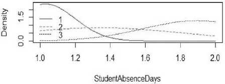
Fig.3. Naïve Bayes method for StudentAbsenceDays.

• B.    Decision Tree

A Decision Tree is a supervised learning algorithm and graphical representation that utilize branching methodology to demonstrate all possible outcomes of a decision .according to certain conditions. In this tree, the internal node symbolizes a test on the attribute, each branch of the tree corresponds to the outcome of the test and the leaf node symbolizes a particular class label means the final decision after all calculations. It is a tree like structure, which begins from root attributes and ends with leaf nodes [19]. We used C5.0 decision tree algorithm for classification purpose. The dplyr, ggplot2, psych, C50 libraries are installed. Loaded the data with read.csv() method. Converted the target variable as factor using as.factor() method. Created the training and testing data. Applied decision tree in training data using c5.0() method. Generated the tree and size of tree is 26. We plotted the tree that shows the track of paths how the decisions are taken and which is displayed in fig. 4.

Equation (7) and (8) are used to predict the loss as 31% and the accuracy as 69% respectively from the testing data in decision tree algorithm.

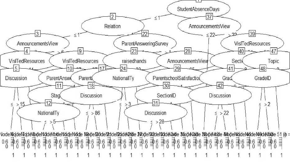
Fig.4. Decision Tree.

• C.    Random Forest

  The Random Forest (RF) is an efficient prediction tool and supervised algorithm in data mining. It makes use of a bagging method to construct forest with more number of trees [22]. It can use for both classification and regression task. The randomForest and caret library is installed. Loaded the data with read.csv() method. Converted the target variable as factor using as.factor() method. Created the training and testing data. Applied random forest in training data using randomForest() method with ntree=500 and mtry=8 (Number of variables tried at each split). Then we printed the random forest and confusion matrix for testing data. The accuracy is 79%, kappa is 0.6798 and Statistics by Classes is shown in table 4.

Table 4. Statistics of Random forest.

Statistics by Class	Class: 1	Class: 2	Class: 3
Sensitivity	0.6800	0.8696	0.8250
Specificity	0.9767	0.7444	0.9583
Pos Pred Value	0.9444	0.6349	0.8919
Neg Pred Value	0.8400	0.9178	0.9293
Prevalence	0.3676	0.3382	0.2941
Detection Rate	0.2500	0.2941	0.2426
Detection Prevalence	0.2647	0.4632	0.2721
Balanced Accuracy	0.8284	0.8070	0.8917

We plotted the random forest with error rate which is shown in fig. 5. Three color lines shows the classes such as Red color line indicates high, green indicates medium, blue indicates low and black line shows the OOBError. Initially errors are high after 100 decision tree there is no significant reduction in error rate.

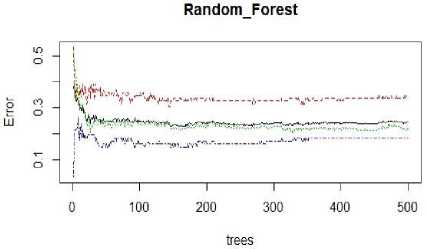
Fig.5. Error rate of Random Forest.

Tuned the mtry on testing data using tuneRF() method with the parameters such as stepFactor=0.5 and ntreeTry=500. OOBError means Out-of-Bag Error. It is used to measure the prediction in Random forest algorithm. OOBError is in y axis and mtry is in x axis and the tuned plot is displayed in fig. 6.

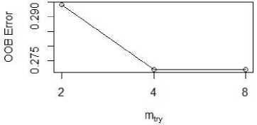
Fig.6. Tuned plot of mtry.

When mtry = 4, OOB error is 27.21% then Searching left reached mtry = 8, OOB error is 27.21%, then Searching right reached mtry = 2 which produced highest OOB error is 29.41%. Number of nodes for the tree is produced with hist(treesize(rf) in fig. 7.

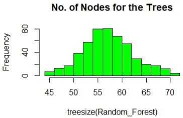
Fig.7. Number of nodes for the trees.

Variable Importance of top 10 variables are calculated using varImpPlot() method and displayed in fig. 8. Mean Decrease Accuracy is how much the accuracy of the model decreases if we drop that particular variable and Mean Decrease Gini is the measure of variable importance according to the Gini impurity index utilized for the computation of splits in trees.

Top 10 - Variable Importance

StudentAbsenceDays

VisiTedResources raisedhands

AnnouncemenisVi ew ParentAnsweri ng Survey

Reiation»

Discussionо grade° -

Topic° - -

Nationally°

10    20    30    40

MeanDecreaseAccuracy

VisITedR esources raised ha nds StudentAbsenceDays

Announcements View

Discussion

ParentAnsweri ngSurvey°

Relation°

GradelDо

PlaceofBirth

0   10 20 30 40 50

MeanDecreaseGini

Fig.8. Plot of top 10 Variable Importance.

The values of all the variable’s MeanDecreaseAccuracy and MeanDecreaseGini are in table 5. The highest MeanDecreaseAccuracy is 46.88396807 for StudentAbsenceDays and highest MeanDecreaseGini is 51.983484 for VisITedResources.

Table 5. MeanDecreaseAccuracy and MeanDecreaseGini of all Variables

Variables	MeanDecrease Accuracy	MeanDecrease Gini
Grade	10.86732288	4.980419
NationalITy	8.46856949	5.194397
PlaceofBirth	6.46343665	5.242359
StageID	6.30999127	3.307117
GradeID	2.72132453	5.800553
SectionID	0.50037601	2.647701
Topic	10.61848248	9.060327
Semester	0.06883277	1.913202
Relation	15.09445779	8.961138
Raisedhands	25.24189048	30.687082
VisITedResources	37.77455810	51.983484
AnnouncementsView	22.53621692	26.034370
Discussion	12.59154998	20.026424
ParentAnsweringSurvey	20.90606528	9.347282
ParentschoolSatisfaction	5.81362717	3.298021
StudentAbsenceDays	46.88396807	28.740246

The Partial Dependence Plot (PDP) is produced using partialPlot() method for VisITedResources attribute and shown in fig. 9. PDP can show the relationship between the target and a feature is linear or complex.

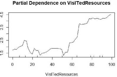
Fig.9. Partial Dependence plot of VisITedResources.

Finally the Multi-dimensional Scaling Plot of Proximity Matrix is generated using MDSplot() method and shown in fig. 10.

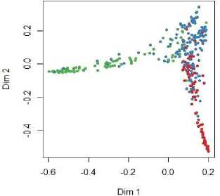
Fig.10. Multi-dimensional Scaling Plot.

• D.    K-Nearest Neighbor

  K-Nearest Neighbor is supervised algorithm; there the destination is already known but the path to reach the destination is not known. The value of k is most important role in predicting the efficiency of the model. The e1071 and caret libraries are used to implement the KNN algorithm in R Programming. We loaded the data with read.csv() method, converted the target variable as factor using as.factor() method. Created the training and testing data. The trainControl() and train() methods are used to form the K-Nearest Neighbors (KNN) model on training data. In train() method we should indicate the method=knn. Then in the step of pre-processing the data with centered (16), scaled (16) and resampling the data with Cross-Validated (10 fold, repeated 3 times) and with tuning parameters. Accuracy was used to choose the optimal model using the highest value. The final value used for the model was k = 19, because when k is 19 the accuracy (0.7418301) and the kappa (0.6060442) values, when K value is 21 and 23 the accuracy and kappa values are decreasing which is shown in table 6.

Table 6. Resampling results across tuning parameters.

K	Accuracy	Kappa
5	0.7300059	0.5869858
7	0.7162507	0.5660492
9	0.7191622	0.5720041
11	0.7141414	0.5629028
13	0.7171717	0.5661146
15	0.7241830	0.5776206
17	0.7349970	0.5945965
19	0.7418301	0.6060442
21	0.7241533	0.5793881
23	0.7281046	0.5860659

The plot of the KNN model clearly depicts the accuracy for all the neighbors (5, 7, 9, 11, 13, 15, 19, 21 and 23) and accuracy is high when the K value is 19 on training data, which is in fig. 11.

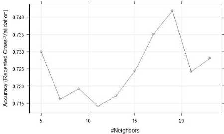
Fig.11. Plot of the KNN model.

The overall statistics of the KNN model is displayed for prediction on testing data and confusion matrix using confusionMatrix() method. The accuracy is 69%, kappa is 0.5217 and Statistics by Classes are shown in table 7.

Table 7. Statistics of KNN model.

Statistics by Class	Class: X3	Class: X1	Class: X2
Sensitivity	0.6429	0.5873	0.8947
Specificity	0.8713	0.7625	0.8762
Pos Pred Value	0.6750	0.6607	0.7234
Neg Pred Value	0.8544	0.7011	0.9583
Prevalence	0.2937	0.4406	0.2657
Detection Rate	0.1888	0.2587	0.2378
Detection Prevalence	0.2797	0.3916	0.3287
Balanced Accuracy	0.7571	0.6749	0.8855

The balanced accuracy for class X3 is 76%, for X1 is 67% and for X2 is 89%.

• E.    Support Vector Machine

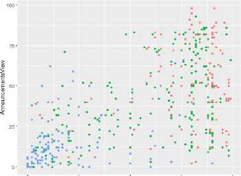
  Support vector Machine is supervised learning algorithm and used for classification, regression and outlier detection. The e1071 and caret, ggplot2 libraries are used to implement SVM model. We installed the packages and loaded the data with read.csv() method. Converted the target variable as factor using as.factor() method. Created the training and testing data. Then we plotted the data for VisITedResources and AnnounmentsView with color=Class using qplot() method in fig. 12. Red dots denote class 1; green dots denote class 2 and blue dots denotes class 3.

О                 25                50                75               100

VisITedResources

Fig.12. Plot of data with 3 classes.

SVM can be implemented with two different kernel types such as linear and radial. First we created the SVM classification plot with kernel type is ‘linear’. The Number of Classes are 3, number of support vectors are 273 (137 =1, 47 =2, and 89=3) and shown the plot in fig. 13.

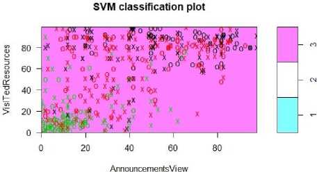
Fig.13. SVM classification plot of linear kernel.

Next we created the SVM classification plot with kernel type is ‘radial’. The Number of Classes are 3, number of support vectors are 367 (180 =1, 75 =2, and 112=3) and shown the plot in fig. 14.

Fig.14. SVM classification plot for radial kernel.

We created the SVM model with Linear as kernel. The overall statistics of the SVM model is displayed for prediction on testing data and confusion matrix using confusionMatrix() method. The overall accuracy is 75%, kappa is 0.6094 and Statistics of SVM model with linear kernel by Class is shown in table 8.

Table 8. Statistics of SVM model with Linear kernel.

Statistics by Class	Class: 1	Class: 2	Class: 3
Sensitivity	0.6667	0.7460	0.8421
Specificity	0.8812	0.7500	0.9619
Pos Pred Value	0.7000	0.7015	0.8889
Neg Pred Value	0.8641	0.7895	0.9439
Prevalence	0.2937	0.4406	0.2657
Detection Rate	0.1958	0.3287	0.2238
Detection Prevalence	0.2797	0.4685	0.2517
Balanced Accuracy	0.7739	0.7480	0.9020

Formed svm_linear_grid for 12 different cost values such as c(0.01, 0.05, 0.1, 0.25, 0.5, 0.75, 1, 1.25, 1.5, 1.75, 2, and 5) using expand.grid() method and resampling with Cross-Validated (10 fold, repeated 3 times) which produced accuracy and kappa result. Resampling results across tuning parameters are displayed in table 9.

Table 9. Resampling results across tuning parameters

C	Accuracy	Kappa
0.01	0.7417391	0.6052831
0.05	0.7424818	0.6052466
0.10	0.7444760	0.6083807
0.25	0.7475045	0.6138000
0.50	0.7515170	0.6200495
0.75	0.7554980	0.6248353
1.00	0.7544879	0.6234508
1.25	0.7564784	0.6268180
1.50	0.7584392	0.6299524
1.75	0.7574291	0.6284510
2.00	0.7584392	0.6299814
5.00	0.7604297	0.6327430

The highest accuracy and kappa value for c is 5. That is accuracy = 0.7604297 and kappa = 0.6327430. Then we plotted the svm_linear_grid with cost as x axis and accuracy as y axis and the plot is shown in fig. 15.

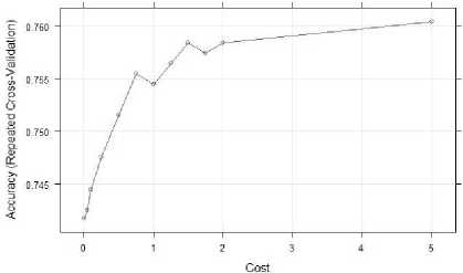
Fig.15. Plot of svm_linear_grid.

Likewise we created the SVM model with Radial as kernel and formed svm_radial_grid with different sigma values such as c(0, 0.01, 0.02, 0.025, 0.03, 0.04, 0.05,0.06, 0.07, 0.08, 0.09, 0.1, 0.25, 0.5, 0.75, 0.9) and C=c(0, 0.01, 0.05, 0.1, 0.25, 0.5, 0.75, 1, 1.5, 2, 5)). Then we plotted the svm_radial_grid with sigma as x axis and accuracy as y axis and the plot is shown in fig. 16. This plot clearly shows that all the cost values are in high accuracy position when the sigma values between 0.0 and 0.1.

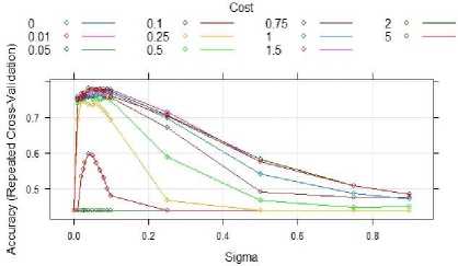
Fig.16. plot of svm_linear_radial.

Finally fine tuned the SVM model. Equation (9) is used to calculate the performance of the model.

epsiIon = ee q(0,1,0.1), cost = 2^Л(2: 3)        (9)

The plot of the performance of the model is shown in fig. 17. The dark region of the plot of the SVM model denotes the better performance.

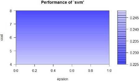
Fig.17. Performance of SVM.

• F.    Deep Neural Network

Neural Network characterizes the neuron as a central processing unit, which plays out a mathematical operation to create one output from a set of inputs. The output of a neuron is a function of the weighted sum of the inputs and the bias [31]. Each neuron plays out an exceptionally straightforward task that includes initiating if the aggregate sum of signal received surpasses an activation threshold. The development of neural networks with huge number of hidden layers is called as Deep Neural Network (DNN). The fig. 18 shows the architecture of DNN.

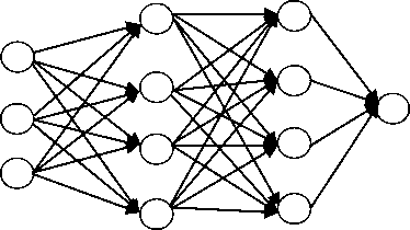
Input Layer Hidden Layer 1 Hidden Layer 2 Output Layer

Fig.18. Architecture of DNN.

There are abundant products and packages are available in the market for deep learning. Some of these are Keras, TensorFlow, h2o, and many others. We used Keras and TensorFlow in R programming.

Terminologies in DNN are Input layer, Hidden layer, Output layer, Weights, Bias, Epoch, Activation functions. There are three layers. The inputs form the input layer, the middle layer(s) which plays out the preparing is known as the hidden layer(s), and the outputs forms the output layer. Epoch is one iteration or pass throughout the development of providing the network with an input and also updating the weight of the network. An activation function is a mathematical operation which converts the input to an output. Types of activation function are linear function, Unit step activation function, sigmoid function, hyperbolic tangent and Rectified Linear Unit (ReLU).

The keras, mlbench, dplyr, magrittr and neuralnet libraries are installed and loaded. Imported the data with read.csv() method. Formed the deep neural network using neuralnet() method with two hidden layers 10 neurons and 5 neurons. We plotted the neural network with the weights. Fig. 19 clearly depicts that input layer with 16 attributes, first hidden layer with 10 neurons, second hidden layer with 5 neurons and output layer is one target attribute with 3 class values.

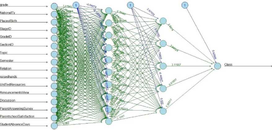
Fig.19. Deep Neural Network.

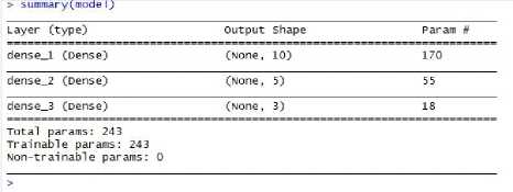
Fig.20. Summary of the DNN model.

Converted the data into matrix and partitioned into the training and testing data using 16 attributes. We formed trainingtarget and testingtarget using the target variable. Normalize the data using colMeans() method. The keras_model_sequential() is used to create the neural network model. Formed two hidden layers of 10 neurons and 5 neurons using layer_dense() with ‘relu’ (Rectified Linear Unit) activation function, and the output layer units=3 (Multi-class classification) with ‘softmax’ activation function. Then we printed the summary of the DNN model using summary(model) method in fig. 20. The DNN model contains information about the layer (type), output shape and the number of parameters. The input layer is passing 16 independent variables; the first hidden layer is 10 neurons, the number of parameters for this layer is 170 that is (16*10) +10. For second hidden layer are 55 that is (10*5) +5. Likewise For the output layer is 18 that is (5*3) +3. Finally the total number of parameters and trainable parameters for the Deep Neural

Network model is 243 produced by summing all the layers parameters (170 + 55 + 18).

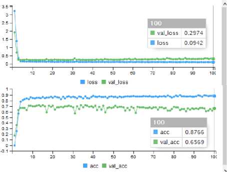
Fig.21. Accuracy and Loss of the model.

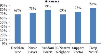
The comparison graph of accuracy for all the six different machine learning algorithms are in fig. 23 and this shows that Deep Neural Network produced high accuracy.

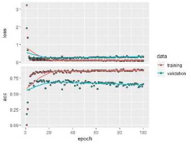
Fig.22. Plot of Deep Neural Network

Compile the model with three parameters such as loss = ‘categorical_crossentropy’, optimizer = ‘adam’, and metrics = 'accuracy'. Fit the model using fit() method with parameters such as training, trainingtarget, epoch=100, batch_size =32, and validation_split=0.3. The accuracy and loss for 100 epochs are in fig. 21.

(С5.0)

Machine Network

Fig.23. Accuracy comparison graph of 6 Machine learning algorithms

The accuracy of training data (acc) and testing data (val_acc), loss of training data (loss) and testing data (val_loss). Predicted the accuracy is 85% which is the highest percentage among all machine learning algorithms. Fig. 22 shows the plot of the Deep Neural Network model.

The confusion matrix is displayed in table 10 for all the algorithms with accuracy.

Table 10. Confusion Matrix of different Machine Learning Algorithms.

S. No.	Machine Learning Algorithms		Predicted				Accuracy
				1	2	3
1	Decision Tree (C5.0)	Actual	1	30	19	0	69%
			2	9	35	8
			3	0	9	33
2	Naïve Bayes		1	33	21	0	73%
			2	5	36	5
			3	1	6	36
3	Random Forest		1	34	2	0	79%
			2	16	40	7
			3	0	4	33
4	K-Nearest Neighbor		1	27	13	0	69%
			2	15	37	4
			3	0	13	34
5	Support Vector Machine		1	28	12	0	75%
			2	14	47	6
			3	0	4	32
6	Deep Neural Network		1	39	8	0	84%
			2	2	43	7
			3	0	4	40

• V.    Conclusion

Predicting the student performance is very important role in educational area so that the analysis of student’s status helps to improve for better performance. Applying data mining concepts and algorithms in the field of education is educational data mining. Machine learning algorithms are applied in the entire field. We proposed the student performance prediction system then trained the model and tested with Kaggle dataset using different machine learning algorithms such as Decision Tree (C5.0), Naïve Bayes, Random Forest, Support Vector Machine, K-Nearest Neighbor and Deep neural network in R Programming. Finally compared the results of six algorithms out of which Deep Neural Network outperformed with 84% as accuracy.