Complexity of Computations with Time Travel

Author: Milad Joudakizadeh, Anatoly P. Beltiukov
Journal: Программные системы: теория и приложения @programmnye-sistemy
Section: Теоретические основания программных систем
Article in issue: 2 (65) т.16, 2025.
Free access
This paper explores a mathematical model of computation that can be interpreted as a computer capable of receiving data from future states of its own computational process. Under certain combinations of input data and programs, such computations may become infeasible due to emerging contradictions or lead to ambiguous outcomes. We investigate programs for which this process is always feasible and yields a unique result. It is demonstrated that, in the absence of computational complexity constraints, such machines can output the value of any recursively decidable predicate within a fixed time after the computation begins—referred to as the response delay time—while the computation process must continue even after the result is produced. When the total runtime of these machines is bounded by a polynomial function of the input size, they precisely recognize languages belonging to the intersection of the NP and co-NP complexity classes, with the same constant response delay time in the aforementioned sense. Possible practical implementations of such a computer are examined, including an analysis of operational protocols leveraging quantum annealing to select the appropriate computational process. It is shown that, with parallelization of the computational process, the class of problems solvable by these machines in polynomial time corresponds to the PSPACE complexity class. Additionally, a mode of operation is studied in which these machines have direct access to input data. In this case, if the runtime is limited to a logarithmic function of the input size, the class of problems solvable by such a parallelized computer encompasses LOGSPACE The findings of this study can be applied to develop new programming principles for nondeterministic computational machines, where data transmission from the future is employed instead of nondeterministic choices.
Turing Machine, Computational Complexity, Recursive Sets, Nondeterministic Computation, Quantum Annealing, Time Machine, Artificial Intelligence
Short address: https://sciup.org/143184481
IDR: 143184481 | UDC: 004.415.2: 519.681 | DOI: 10.25209/2079-3316-2025-16-2-3-54
Сложность вычислений с путешествиями во времени
Эта работа рассматривает математическую модель вычислений, которая может интерпретироваться как компьютер, способный получать данные из будущих состояний своего вычислительного процесса. При определённых сочетаниях входных данных и программ такие вычисления могут становиться невыполнимыми из-за возникающих противоречий или приводить к неоднозначным результатам. Мы исследуем программы, для которых этот процесс всегда выполним и даёт однозначный результат. Показано, что при отсутствии ограничений на вычислительную сложность такие машины могут выдавать значение любого рекурсивно разрешимого предиката через фиксированное время после начала вычисления — время задержки ответа (при этом процесс вычисления должен продолжаться и после получения ответа). Если общее время работы таких машин ограничить полиномами от размера входных данных, то эти машины будут распознавать в точности языки, принадлежащие пересечению классов NP и co-NP, за постоянное время задержки ответа в таком же смысле. Рассматриваются возможные реализации такого компьютера на практике, включая анализ возможных протоколов работы с использованием квантового отжига для выбора нужного процесса. Показано, что при распараллеливании вычислительного процесса класс задач, решаемых рассматриваемыми машинами за полиномиальное время, соответствует классу PSPACE. Кроме того, исследуется режим работы, при котором эти машины имеют прямой доступ ко входным данным. В этом случае, если время работы ограничено логарифмом от размера входных данных, то класс задач, решаемых таким параллельно работающим компьютером, содержит LOGSPACE. Результаты данного исследования могут быть использованы для разработки новых принципов программирования недетерминированных вычислительных машин, в которых вместо недетерминированных выборов используется передача данных из будущего.
Text of the scientific article Complexity of Computations with Time Travel
This article presents an unconventional perspective on computational processes. What happens if a machine is allowed to peek into its own future and use this information to make decisions in the present? This idea, which at first glance seems inherently paradoxical, lies at the heart of the computational model under investigation—Turing machines with a backward-in-time communication channel. This model not only redefines the understanding of time in computation but also raises fundamental questions about causality and the interaction between past and future in computational processes.
Our machine is defined in such a way that it can receive information from future states of its computational process. This model represents a theoretical framework that introduces new ways of organizing computations. It allows obtaining the result of a complex computation before its completion and using this information. As with any time travel scenario, complications arise: transmitting data from the future may lead to contradictions and ambiguities.
In this article, we focus on cases where such problems can be avoided and demonstrate how this model can be implemented and applied to solve complex problems. This approach offers an alternative computational paradigm that connects time, causality, and computation, enabling new problem-solving strategies.
One of the results is that such a machine can compute the value of any recursively enumerable predicate in constant time. This means that tasks requiring significant time in classical models can be solved almost instantaneously (although the computational process itself must continue, and its total duration may still be substantial).
We also prove that if the total runtime of such machines is bounded by polynomials in the input size, they can recognize all languages in the intersection of NP and co-NP . These results indicate that the proposed model is not only theoretically interesting but also possesses significant computational power.
We also consider a modification of the machine that enables parallel data processing. It is shown that in this case, the class of problems solvable by such machines in polynomial time corresponds to PSPACE (i.e., polynomial time on the new machines is equivalent to PSPACE on ordinary Turing machines).
Another modification involves adding a mechanism for direct access to input data by addressing cells of the input tape using a special address tape. In this case, with runtime limited logarithmically in the input size, the class of problems solvable by our parallel computer includes LOGSPACE (here, LOGTIME also translates into corresponding space complexity). It is worth noting that this mode of operation does not entail excessive complexity and is feasible on conventional computers for reasonable input sizes.
From a practical standpoint, our work introduces new programming mechanisms. Instead of complex nondeterministic choices, which can be difficult to comprehend, we propose using data from the future, making the computational process more intuitively understandable. We also explore possible implementations of this model, including deterministic backtracking and quantum annealing.
In the first approach, systematic backtracking ensures that all possible paths are explored to prevent paradoxes. In the second approach, quantum adiabatic machines simultaneously explore multiple states of the computational process, selecting a self-consistent sequence of actions.
Thus, we propose a model that expands our understanding of computational processes and provides new approaches to programming.
1. Related Work
Over the past few decades, the idea of utilizing temporal paradoxes and time-traveling data transmission has attracted attention in theoretical computer science and physics. Many researchers have explored the possibility of extending classical computational models by incorporating mechanisms that allow information to be retrieved from the future, which is hypothesized to redefine traditional views on computational resources and complexity.
In the seminal work by Cook [1] , the concept of NP -completeness was introduced, laying the foundation for further research in computational complexity and the reducibility of various problems to a universal problem. Expanding on these ideas, R. M. Karp [2] analyzed the reducibility of combinatorial problems, demonstrating that many seemingly disparate problems are interconnected.
The classic work by Garey and Johnson [3] became a fundamental reference for researchers studying computational complexity, presenting a wide range of NP-complete problems and serving as a starting point for analyzing the limitations of traditional computational models.
In recent years, significant attention has been devoted to models that leverage physical effects to solve complex computational problems. Aaronson [4] investigated the potential of quantum computing for solving traditionally hard problems, showing that quantum methods can provide substantial advantages over classical algorithms.
Deutsch [5] introduced the concept of a universal quantum computer, marking a ma jor milestone in quantum computing and influencing subsequent research on hybrid computational models.
Regarding models that violate classical causality, substantial contributions have been made in studies related to closed timelike curves (CTCs). Brun [6] demonstrated that the use of CTCs can significantly accelerate problem-solving. Moreover, Aaronson and Watrous [7] established the equivalence of quantum and classical computations in the presence of CTCs, highlighting the potential of such models to expand computational capabilities.
Beyond classical approaches, the idea of integrating time-travel-based data transmission with complexity theory has sparked interest. The works of Papadimitriou [8] and Arora and Barak [9] provide a deep analysis of the structure of computational problems, including the relationship between NP and co-NP classes. These studies serve as a foundation for analyzing how nonstandard computational models that utilize future data transmission can solve problems that are difficult for traditional models.
Classical works on quantum computing, such as the book by Nielsen and Chuang [10] , as well as the algorithms of Grover [11] and Shor [12] , illustrate how quantum methods can significantly accelerate the solution of certain problem classes.
More recent studies, such as those by Harrow and Montanaro [13] and Iqbal et al. [14] , confirm the practical significance of quantum algorithms for solving complex computational problems.
An important aspect of this field is the concept of time-travel-based data transmission, which allows machines to predict their future states and use this information to adjust current computations. In this context, the work by Orlicki [15] explores a model of time-traveling machines and examines the problem of self-consistent halting. This approach extends traditional models, offering new perspectives on the interaction of temporal flows in computation.
Furthermore, Godel’s contribution [16] demonstrated the theoretical possibility of closed timelike curves in cosmological solutions, providing additional physical justification for computational models involving future data transmission.
Studies by Bacon [17] and Wolpert [18] indicate that physical constraints on future prediction and feedback between temporal states significantly influence computational processes.
Finally, experimental research, such as the work by King et al. [19] , shows that quantum systems with thousands of qubits can already simulate complex physical phenomena, raising hopes for the practical feasibility of computational models that exploit time-travel effects.
Thus, these works illustrate that the idea of future data transmission and temporal loops in computation has strong theoretical and practical foundations. Our time-traveling computation model naturally fits into this context, offering a fresh perspective on computational complexity and enabling the solution of problems that are intractable for traditional models.
2. Structure and Features of the Turing Machine with Time Data Transmission Channel
This section describes the construction of a Turing machine equipped with a time data transmission channel. This model extends the classical Turing machine by including a mechanism that allows data to be transmitted to previously executed steps of the computational process and to receive data transmitted from future steps. Let us consider the structure and features of such a machine.
-
2.1. Main Components of the Machine
The Turing machine with a time data transmission channel is a multitape machine (with one head for each tape) and includes the following elements:
Input Tape: This tape contains the input word that needs to be processed.
At the beginning of the machine’s operation, the input data is written to this tape.
Output Tape: The result of the machine’s operation is recorded on this tape. For a recognition machine, the result can be represented as a binary value: 0 (no) or 1 (yes).
Multiple Working Tapes for performing necessary computations.
Communication Tape (Connection Tape): A special tape designed for transmitting data in time. The machine can write data to this tape for sending to the past and receive data from the future. To send and receive data, the machine must transition to special states for data transmission and reception, respectively.
Address Tape for Transmitted Data: This tape records labels that allow data to be retrieved by referencing these labels in requests. Special machine states are used for data transmission and retrieval.
In the transmission state, the contents of the communication tape along with the label are sent to the time data transmission channel. If data with such a label has already been sent earlier, it is considered that an error has occurred during the machine’s operation.
In the reception state, the communication tape receives data from the transmission channel associated with the specified label. If such data was not found in the future, it is also considered that an error occurred during the machine’s operation. For solving recognition tasks where errors may occur during operation, usage is prohibited. Tape Alphabets: Each tape has its own alphabet of symbols that can be written on it.
Control Unit: At each step of operation, the control unit can be in one of the states of the state alphabet. The following special states are distinguished:
initial state (in which the machine begins the computational process), final state (in which the machine’s operation is completed), data transmission state (to which transitioning sends data with the specified label to the data transmission channel), data reception state (to which transitioning receives data from the data transmission channel with the specified label), output state (to which transitioning sends the contents of the output tape to the outside world while the machine continues its operation), considering that the machine operates with a single write to the output tape, meaning that a repeated transition to the output state is an error in the machine’s operation.
Program: A function (table) that maps the machine’s state and the symbols visible to the heads on each tape to a new state, new symbols to be written on the tapes, and the directions of head shifts.
Past
Future
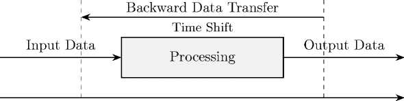
Figure 1. Schematic of reverse-time data transfer in a Turing machine with closed timelike curves
Time
Computation Time: A sequence of steps. Each step performs one machine command or transmits/receives one symbol through the time data transmission channel (i.e., transmitting a long word to the data transmission channel takes as many steps as the length of that word). For a recognition machine, computation time must be finite.
In diagram Figure 1, the process of data processing with the possibility of transmitting information from the future to the past through a time shift is shown, implemented by closed time-like curves in Kerr metric.
-
2.2. Features of the Machine’s Operation
-
2.3. Temporal Aspects of the Machine’s Operation
The operation of the Turing machine with a time data transmission channel has several distinctive features:
Output of the result before the completion of computations: The machine can output the result to the output tape before the computation process is completed. This leads to a separation of two concepts of time:
response delay time, total computation time.
Uniqueness and definiteness of computations: Due to the ability to obtain data from the future, the operation of the machine may become ambiguous or indeterminate. For example, ambiguity arises if the machine, having received some data from the future, writes the same data with the same label, which may lead to non-determinism in the process and, consequently, to different final results, depending on which data ends up being read and written. If the machine, having read data with one label, then necessarily writes different data with the same label, a contradiction arises, making the process impossible, leading to indeterminacy. A machine is considered to recognize a certain property of the input data (i.e., computing the characteristic function of some set) if its operation is defined for all input data and the result is unique.
Programmability: At the end of the article, we will describe tools of algorithmic languages that will allow programming such actions not only for Turing machines but also for other computers.
A key feature of the machine is the ability to obtain data from the future, which leads to the following temporal effects:
Constant response delay time: Thanks to the mechanism of time data transmission, the machine can produce a simple result ( YES or NO in constant time, regardless of computational complexity.
Total computation time: Despite the constant response delay time, the total computation time may be significantly longer, as the computation process must continue even after the result is output.
-
2.4. Explanation of Ambiguity and Indeterminacy
To illustrate the ambiguity and indeterminacy in the operation of the machine, consider the following example. Suppose the machine queries one bit from the future and chooses a branch of computations based on its value. If the bit value of 1 is received, the machine follows the first branch; if a value of 0 is received, it follows the second branch. Ambiguity in the computation process arises if, in each branch, the machine writes the same bit with the same label to the communication tape. This creates two possible paths of computation. It is important to distinguish between the ambiguity of computation and the ambiguity of the result. In an ambiguous computation process, the result may turn out to be the same.
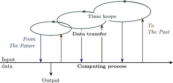
Figure 2. Schematic of temporal data flow in a Turing machine with closed timelike curves
If the machine reads one bit from the future and tries to write a contradictory bit to the communication tape with the same label, a contradiction arises, making such computation impossible.
Combinations of these situations may lead to some branches of the computation process, arising from internal ambiguity, subsequently becoming contradictory and thus being discarded. Only non-contradictory branches will remain. It may happen that all remaining non-contradictory branches lead to one final result. If this always occurs, we will consider such a machine correct for solving the recognition problem.
Thus, the described situations may lead to the following: ambiguity, if several branches of computations end with different results, indeterminacy, if no branch can complete without contradictions.
This demonstrates how the use of data from the future can affect the computational process.
3. Capabilities of Machines with Time Data Transmission
The scheme of data transmission in time for a Turing machine with closed time-like curves is presented in Figure 2.
It shows the main stages of information processing, the feedback mechanism through time loops, and the direction of data transmission.
In this section, we examine the computational capabilities of the Turing machine with a time data transmission channel. We present two theorems that demonstrate how the use of data from the future affects the computational complexity and classes of problems solvable by such a machine. These theorems show that the proposed model possesses properties that allow solving problems inaccessible to classical computational systems.
-
3.1. Recognition of Decidable Sets
-
3.2. Recognition of Sets in NP∩ co-NP
Theorem 1 . A Turing machine with a time data transmission channel recognizes all recursively decidable sets with constant response delay time.
Proof. The proof is based on the machine’s ability to use data from the future to predict the results of computations. Let us recognize the membership of input strings in a given recursively decidable set. There exists a standard recognizing Turing machine for this set. From this machine, we will construct the required Turing machine with a time data transmission channel that will operate as follows.
At the start of its operation, the machine requests the contents of the communication tape labeled 0. This value is output as the result of its operation. Then, the process of the standard Turing machine recognizing membership in the given set is initiated. When the recognition is complete, its result is transmitted to the past with the label 0. This ensures that in the past, the machine provided the correct result.
Now, let us assume we have the original machine with a time data transmission channel that recognizes the membership of input strings in some set. By definition, the total running time of such a machine is always finite. We will construct a new standard Turing machine that recognizes membership in this set, which enumerates all possible strings that could serve as a partial protocol of the original machine’s operation (chains of instantaneous descriptions), in order of their lengthening.
The machine checks for each string whether it is a correct completed protocol of the original machine’s operation. As soon as such a protocol is found, the result of the original machine’s operation is output as the result of the new machine. Since the operation of the original machine, by definition, is definite and unique, the new machine always provides the correct answer regarding the membership of the input string in the given set. □
Theorem 2 . A Turing machine with constant response delay time and polynomial total computation time recognizes exactly all sets in NP ∩ co-NP
Idea of the Proof. By interpreting the reception of data from the future as branching into several paths, we construct a machine that operates in polynomial time and ensures the consistency of results across all branches of computations.
4. Proof of Theorem 2
In this section, we will present the proof of Theorem 2 , formulated in the previous section. First, we will reformulate the operation of our machine in terms of nondeterministic computations. This will allow us to transform the operation of our machine into the operation of standard nondeterministic Turing machines and vice versa. Since the mechanism for transitioning to constant response delay has been described in the proof of the previous theorem, we will initially prove Theorem 2 without mentioning this, which we will do.
-
4.1. Transition to Nondeterministic Computations
The idea is to interpret the reading of each data symbol on the communication tape, received from the future by some label, as branching in the computation process. Each branch corresponds to one of the possible values of that symbol. When the machine reaches the moment in time denoted by this label, it checks whether the assumed read symbol matches the transmitted one. If the value of the symbol recorded in the communication tape cell matches the expected value in the current branch, the computations continue. Otherwise, the computation branch ends due to a contradiction.
A correct recognizing machine must provide the same answers (either 0 — NO or 1 — YES on all consistently terminating branches for a given input word. Next, we will transform our original machine with time data transmission into a nondeterministic one, as shown above, and then split it into two nondeterministic Turing machines, handling the aforementioned contradictions as follows:
-
(1 ) The first machine accepts the recognized set, returning 1 when the original machine outputs 1, and returns 0 in all other cases (including contradictions).
-
(2) The second machine accepts the complement of this set, returning 1 when the original machine outputs 0, and returns 0 in all other cases (including contradictions).
-
4.2. Constructing a Machine with Time Data Transmission from Nondeterministic Machines
Thus, if the original machine with time data transmission outputs YES then the first of the resulting machines outputs YESon some branches of the computation, while the second always outputs NO Conversely, if the original machine outputs NO then the first always outputs NO while the second outputs YESon some branches of the computation. Thus, the first of the constructed deterministic machines accepts the recognizable set itself, while the second accepts its complement. It is easy to see that the polynomial time bound is preserved in the specified transformation, as all performed restructurings give at most polynomial slowdown. So, if the original machine recognized the given set in polynomial time, the newly constructed machines operate in the same time. This means that the originally recognized set belongs to NP ∩ co-NP
The reverse statement is also true: if there exist two nondeterministic machines, bounded by polynomial time, one of which accepts some set and the other accepts its complement, we can construct a single machine with time data transmission from the future that recognizes this set and operates in polynomial time. This machine operates as follows:
(1) At the beginning of the process, it guesses which of the two nondeter-ministic machines to run.
(2) It then executes the chosen machine.
(3) If the first selected machine outputs 1, the computation branch ends with the result 1.
(4) If the first selected machine outputs 0, the computation branch leads to a contradiction.
(5) If the second selected machine outputs 1, the computation branch ends with the result 0.
(6) If the second selected machine outputs 0, the computation branch leads to a contradiction.
4.3. Constant Response Delay Time
5. Implementation Questions5.1. Deterministic Backtracking
By assumption, exactly one of these machines must yield a positive result. Thus, our machine always provides a definite answer: either 1 or 0.
Constant response delay time is achieved because the decision about the result of the computations is made at the very beginning of the process. The machine requests data from the future and uses it to immediately output the answer. Meanwhile, the computation process must continue. □
This section discusses possible approaches to the practical implementation of a Turing machine with a time data transmission channel. Although such a machine is a theoretical construct, it can be emulated using existing computational methods and technologies. The main approaches to implementation include deterministic backtracking, annealing methods, particularly quantum annealing. Each of these methods has its own features and limitations, which are discussed below.
One of the simplest ways to implement a machine with data transmission from the future is to use deterministic backtracking on a conventional computer. In this approach, the computation process is modeled as a tree of possible states, where each branch corresponds to one of the possible values of the symbol received from the future.
Working Principle :
-
(1 ) At each step of the computation, when reading a data symbol from the communication tape, the machine checks all possible values of that symbol.
-
(2) If the chosen value leads to a contradiction, the system returns to the decision point and tries the next value.
-
(3 ) The process continues until a consistent solution is found or all possible values are exhausted.
Advantages :
-
• Simplicity of implementation on existing computational platforms.
-
• Ability to use standard search algorithms with backtracking.
Disadvantages :
-
• High computational complexity, especially for problems with a large number of branches.
-
• Exponential growth of computation time as the depth of the decision tree increases.
-
5.2. Annealing Methods
Annealing methods represent a more complex approach to implementing a machine with time data transmission. In this case, the computation process is viewed as a whole structure (time unfolds in space). Then, a search is performed for the state of this structure with the lowest energy, where energy corresponds to the number of contradictions in the system.
Working Principle :
-
(1 ) Initially, the system is in an excited state with a high energy level, corresponding to the presence of many contradictions.
-
(2) Gradually, the system cools down, transitioning to states with lower energy.
-
(3) If a state with the lowest energy (without contradictions) is reached during the annealing process, the process is considered successful.
-
(4) If the lowest energy is achieved for only one answer (0 or 1), the result is considered final.
Advantages :
-
• Ability to find the global energy minimum even in complex systems with many local minima.
-
• Efficiency for problems where contradictions can be mitigated or eliminated during optimization.
Disadvantages :
-
• Requires significant resources to reach a state with minimal energy.
-
• Does not guarantee finding the optimal solution in polynomial time.
-
5.3. Quantum Annealing
Quantum annealing is a promising method for implementing a machine with data transmission from the future, based on the use of quantum devices. This method utilizes the effect of quantum tunneling to find states with the lowest energy.
Advantages :
-
• Potentially high speed of finding solutions due to quantum effects.
-
• Ability to solve problems that are difficult for classical computers.
Disadvantages :
• The speed and computational efficiency of quantum annealing are not yet fully understood.
• Existing quantum devices are limited in memory capacity and noise levels, complicating their use for complex tasks.
5.4. Summary
6. Constructive Recognizers: An Example of Solving a Problem with a Time Data Transmission Machine
6.1. Non-constructiveness of Classical Recognizers6.2. Constructive Problems in the Class NP ∩ co-NP
6.3. Example: Checking for a Non-trivial Divisor
Prospects : Despite current limitations, quantum annealing remains a promising direction for experimentation. Existing quantum annealing machines, such as those from D-Wave (see, for example, [19] ), are already suitable for research and can be used to explore the possibilities of implementing machines with data transmission from the future.
The implementation of a Turing machine with a time data transmission channel is possible using various approaches, including deterministic backtracking, annealing methods, and particularly quantum annealing. Each of these methods has its advantages and limitations, and the choice of a specific approach depends on the characteristics of the problem being solved and the available computational resources. Quantum annealing, in particular, remains a promising direction, although its practical efficiency requires further study.
Classical recognition algorithms are usually non-constructive: they provide only a binary answer (YES or NO without explaining the result.
For example, when asked whether there exists a y that satisfies the condition P(x,y) such algorithms merely confirm or deny the existence of such a y , without providing the actual object y upon a positive answer or proof of its absence upon a negative one. This limits their use in tasks where justification of the solution is required.
A Turing machine with a time data transmission channel allows the implementation of constructive recognizers that provide not only an answer but also a certificate—proof or witness of the result. We consider symmetric problems in the class NP П co-NP, where the property Q(x) is true if there exists a certificate y such that Q 1 (x,y), and false if there exists a certificate z such that Q o (x, z), with the sizes of y and z polynomially bounded relative to | x | .
Consider the problem of determining whether the number x has a non-trivial divisor y such that 1 < y < d (the threshold d is given). This property Q(d,x):
-
• If Q(d, x) = 1, then the certificate is the divisor y, verified by division in polynomial time.
-
• If Q(d, x) = 0, then the certificate is the factorization of x into prime factors, all > d , verified in polynomial time (for example, using the Miller test [20] under the assumption of the generalized Riemann hypothesis).
-
6.4. Implementation on a Time Data Transmission Machine
The constructive recognizer on a time data transmission machine works as follows:
-
(1 ) Receiving Data from the Future :
-
• In the first step, the machine requests a pair (b, C) with label 0, where b G { 0,1 } is the answer, and C is the certificate (divisor or factorization).
-
• The answer b is immediately written to the output tape (if no fixed delay response is required, the certificate can also be issued, making the recognizer constructive).
-
(2 ) Certificate Verification :
-
• If b = 1, it checks that C = y divides x and 1 < y < d.
-
• If b = 0, it checks that C is a factorization of x into prime factors > d, and their product equals x.
-
(3 ) Self-consistency :
-
• After verification, if the certificate is correct, then (b, C ) is written to the communication tape with label 0.
-
• If incorrect, a contradiction is created, and the computation branch is discarded.
It is easy to see that this machine operates in polynomial time.
Execution Example :
Input : x =15, d = 4.
Step 1 : Import (1, 3) from the future, output 1.
Step 2 : Check: 15 ^ 3 = 5, 1 < 3 < 4, correct.
Step 3 : Transmit (1,3) with label 0, self-consistency achieved.
Input : x =17, d = 4.
Step 1 : Import (0, { 17 } ), output 0.
Step 2 : Check: 17 is prime (Miller test), 17 > 4, correct.
Step 3 : Transmit (0, { 17 } ), self-consistency achieved.
-
6.5. Features and Advantages
Linearity : The process is deterministic.
Instant Response : The answer is available in the early steps due to data transmission from the future.
Transparency : If a certificate is issued, it makes the result interpretable, enhancing the clarity of the computations.
Start
End
|
(b,C ) |
|
|
Check C |
Output b
Time
Figure 3. Scheme of the Constructive Recognizer’s Operation
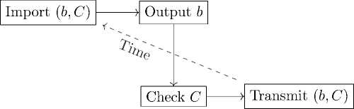
Figure 4. Flowchart of the Process
Figure 3 presents a scheme of the constructive recognizer’s operation: data (b, C ) is transmitted from the end of the computations to the beginning for immediate output and subsequent verification. The flowchart of the process from importing the result to verification and self-consistent data transmission is shown in Figure 4.
7. Actions for Time Data Transfer
To transform a conventional programming language into one that supports time data transfer, it is necessary to add two new operations: transferring data to the past and receiving data from the future. These actions allow the machine to interact with both future and past states of the computational process, providing new programming capabilities. In this section, we will examine these actions and their role in organizing computations with time data transfer.
-
7.1. Action of Transferring Data to the Past
The action of transferring data to the past allows the machine to record data at a specific moment in time, which can be used in previous computations. This action is formalized as follows:
Formal Description :
-
• transfer(l, d): transfers object d to the moment in time l.
-
• l — the label of the moment in time for which the data is being transferred.
-
• d — the object being transferred (e.g., bit, number, or string).
Working Principle :
-
(1 ) The machine records object d in the time data transfer channel with the timestamp l .
-
(2) The data becomes available for use in previous steps of computations related to the moment in time l .
-
(3) If a record with label l already exists, an error occurs.
-
7.2. Action of Receiving Data from the Future
Example : If the machine executes the action transfer (1,1), the value 1 is transferred with label 1. In previous computations related to 1, this value can be used for decision-making.
The action of receiving data from the future allows the machine to obtain data from a specific moment in the future, making it possible to use future information in current computations. This action is formalized as follows:
Formal Description :
-
• accept (l): accepts data from the moment in time with label l.
-
• l — the name of the moment in time from which data is requested.
Working Principle :
(1) The machine requests data from the time data transfer channel with timestamp l.
(2) If the data exists, it is returned and can be used in current computations.
(3) If the data is absent, an error occurs.
7.3. Interaction of Data Transfers
7.4. Summary
8. Parallelization of the Computational Process
Example : If the machine executes the action accept (1), it receives the value d, which was transferred with label 1 using the action transfer (1, d). This value can then be used for decision-making in current computations.
The actions of transferring and receiving data work together, ensuring a connection between current and future states of the computational process. This interaction allows the machine to obtain data from the future for decision-making in current computations. It is important to note that the volume of data transferred through time is a significant indicator of the complexity of the computation. For example, when implementing a backtracking process, the runtime slows down exponentially with a binary indicator of the volume of data in bits, as for each bit of data, it effectively requires entering two branches of computation. Similar complexities arise in annealing methods.
The actions of transferring and receiving data through time are key elements of our computational model. In principle, we can incorporate these capabilities into any programming language, transforming it into a language for controlling a machine with data transfer from the future to the past. These tools provide new opportunities for creating intuitive computational systems.
This section describes a parallel machine with time data transfer—an extension of our machine with an additional capability aimed at increasing its computational power: executing another instance of the machine with specific input data. The input string for the new process is placed on a special argument tape. The parallel process is initiated when the machine transitions to a special state for starting a parallel process. The new process begins with a special initial state of the subprocess. Initially, the new process runs until it reaches a state where it outputs a result (while the old process waits). This result is then transferred from the output tape of the new process to the argument tape of the old process. Both processes then continue to execute in parallel, with the old process no longer interacting with the new process. The parallel execution of the new process is necessary for transferring data to the past within it, ensuring the correctness of the result produced by this process.
The new process can be started as many times as necessary, either by the main process or by spawned subprocesses. Since subprocesses can launch their own subprocesses in parallel and independently, the number of subprocesses can grow exponentially as the machine operates in parallel mode.
The total parallel runtime of the machine is considered to be the time until all parallel processes complete, as if they were executed synchronously, step by step.
Theorem 3 . On a paral lel machine with time data transfer, the operation of a conventional Turing machine with polynomial memory can be modeled in polynomial time (which corresponds to the complexity class PSPACE ).
Proof. Consider a Turing machine with a known estimate of its capacity complexity in the class PSPACE . We will perform the following steps:
(1) First, estimate the runtime of this machine (exponential in the volume of memory).
(2) Launch a subprocess to model the operation of the machine for half of this time (the modeling time is passed to the subprocess along with the initial configuration of the process).
(3) After obtaining the result and allowing the subprocess to continue forming it in the future, immediately launch a new subprocess to model the operation of the original machine for the remaining half of the allocated time, passing this subprocess the configuration obtained from the first subprocess.
(4) Output the result.
(5) The subprocesses continue working in a similar manner until the allocated time converges to a predetermined constant.
9. Direct Access to Input Data
It is easy to see that the depth of subprocess calls here is polynomial, and the total parallel runtime is also polynomial. This completes the proof of the theorem. □
Theorem 4 . The operation of a parallel machine (with time data transfer) in polynomial time can be modeled by a conventional Turing machine with polynomial memory.
Proof. The reverse statement follows from the fact that the operation of such a parallel machine can be modeled on a conventional Turing machine using polynomial memory. This is achieved by sequentially executing all launched processes, as they do not interact with each other. Since the total parallel time of the modeled machine is polynomially bounded, the depth of subprocess calls is also polynomially bounded. Thus, the total memory volume for modeling also remains polynomial. This proves the theorem. □
In this section, we modify the model of our machine by adding the capability to work with large data through direct access to the cells of the input tape. By large data, we mean data that cannot be sequentially examined within the current time constraints. The direct access mechanism allows for quick access to remote cells, overcoming the specified limitation. This is achieved as follows: a special address tape is introduced, on which the binary representation of the cell number on the input tape is recorded. The input tape head instantly moves to the specified cell. No other mechanisms for moving this head are provided. We assume that all launched subprocesses work with the same input data. Thus, we have defined a parallel machine with time data transfer and direct access to input data.
If we replace PSPACE with LOGSPACE in the previous section, we obtain the following theorem.
-
Theorem 5 . On a parallel machine with time data transfer and direct access to input data, the operation of a conventional Turing machine with logarithmic memory (LOGSPACE) can be modeled in logarithmic time (LOGTIME).
Proof. It is similar to the proof of Theorem 3, but with the replacement of polynomial constraints with logarithmic ones. Since access to input data occurs in constant time, the total execution time remains logarithmic. □
The reverse statement is problematic since direct modeling of logarithmic time on our machine using a conventional Turing machine requires a memory volume polynomial in the logarithm of the size of the original data. However, a similar approach can be used to prove the following theorem.
-
Theorem 6 . The class POLYLOGTIME on a parallel machine with time data transfer and direct access to input data coincides with the class POLYLOGSPACE for conventional Turing machines.
Proof. The proof is based on the fact that the operation of our machine with direct access can be modeled on a conventional Turing machine using polylogarithmic memory. Thus, the total modeling time remains polylogarithmic. □
Conclusion
This work presents a fundamentally new computational model that expands classical representations of computational processes through the mechanism of transferring data across different moments in time. The main results of the research are as follows:
-
(1 ) Complexity Classes and Time Constraints : It has been proven that a machine with data transfer from the future, without time constraints, recognizes exactly the decidable sets with a constant response delay. Under polynomial time constraints, the model corresponds to the class of problems in the intersection of NP and co-NP . These results demonstrate how controlled violations of causal order can assist computations.
-
(2) Parallelization and Space Complexity : The extension of the model to allow the launching of subprocesses that inherit input data enables the coverage of the PSPACE class in polynomial time, demonstrating how time complexity transforms into space complexity.
-
(3) Direct Access and Data Processing Efficiency : The modification with addressable access to the input tape and logarithmic time complexity ensures compliance with the LOGSPACE class, which is particularly relevant for large data processing tasks. This result is supported by the mechanism of instant movement of the input tape head, eliminating linear delays.
-
(4) Practical Implementation : Two approaches to the practical implementation of the model are proposed:
-
• Deterministic Backtracking — a systematic search for self-consistent computational tra jectories;
-
• Annealing Methods (including quantum systems) — searching for states with minimal energy of contradictions.
Experiments with quantum annealers, such as D-Wave, could be the next step in assessing the physical realizability of the model.
The prospects for further research encompass both theoretical and practical aspects:
-
• Optimization of the volume of transmitted data to reduce computational load;
-
• Development of specialized programming languages with operators for time data transfer;
-
• Analysis of the connection with quantum computing.
This work is relevant not only for theoretical computer science but also for interdisciplinary research. It demonstrates that the connection of states in time may be the key to solving problems inaccessible to traditional systems. The proposed model could serve as a bridge between complexity theory and physical realizations, opening new possibilities for algorithms.
