Computational Fluid Dynamics Verification and Noise Prediction of Ramjet with Wedge-shaped Flame Holder

Published Online April 2012 in MECS DOI: 10.5815/ijisa.2012.03.01

It is well-known the ramjet principle was originally developed in 20th century by a French engineer, Rene Lorin, to overcome other engines’ shortages such as the complexity, lightweight, small volume, and low thrustweight ratio, and so on. So, most of the nations around the world are concerned about the various methods of improving the performance and enter the research of the backwards facing step or cavity flame holder to gain a great breakthrough in the ramjet engine, actively. However, future studies have highlighted to limit those methods is the lack of efficient combustion capacity. Thus, this phenomena has led widespread attention and better development in the wedge-shaped flame holder, which involving the roles of flame stabilization and mix improvement, and achieved more satisfactory results in existing types of the ramjet engine [1-5].With developing the flame stabilization technology and studies on this area, exploring noise, which caused by flow and combustion are vital because the problem is becoming increasingly prominence. There are currently lots of articles focus on outside noise and developing variety of methods to preserve the environment. In contrast, the inside parts are ignored.

This paper is aimed at exploring the rules of the noise spatial distribution within the combustion chamber. In Section 2, different turbulence models, time step sizes and meshes are selected for the same initial condition and the results, in terms of velocity and temperature of the chamber at given condition, are obtained and precisions of these computing models are compared. In light of these results, a conclusion about the calculation method is determined. In Section 3, noise prediction results under combustion and cold flow condition are presented and compared. The conclusions are contained in Section 4.

• II.    Flow Verification

Under assuming the gas meets the ideal gas equation of state and ignores the two-phase flow, the mesh of half of the ramjet with the wedge-shaped flame holder, which shown in Fig.1, is established according to the characteristics and size of the workload. Therefore, the flow within the chamber is the formula using the Navier-Stokes equation, based on the conservation of mass, momentum and energy. The mathematical expression can be defined as [6-7]:

д д         д 56

Where Φ is arbitrariness independent variable and Г Φ is transport coefficient, S Φ and S PΦ are gas source term and the term between gas phase and particle, respectively. S is sum between S Φ and S PΦ .

Figure 1. Computational model

Depending on Oevermann’s experiments give the detailed distribution of primary parameters, such as velocity, temperature, etc., those results are employed to verify the accuracy of the numerical model. The two inlet boundary conditions are determined as the following illustration, which listed in Table.1 [8].

TABLE 1. BOUNDARY CONDITIONS

Parameter	Air	Hydrogen
Total pressure (Pa)	782445	189293
Total temperature (K)	612	300
Velocity (m/s)	757	1200
Y H2	0.000	1.000
Y N2	0.736	0.000
Y O2	0.232	0.000
Y H2O	0.032	0.000

Where Y is the mass fraction and the subscripts are species.

It is an obvious truism the calculation methods must be choosing carefully to gain credible data from the numerical computation, so the parameters must consider them in detail. Previous studies have illustrated that one has to make combustion simulations using practicable transport models and compare the experimental observable with the theoretical predictions to extract the information about supersonic flow within the ramjet. Considering many of the recommendations in the literature, the finite rate model is used to flow validation based on the analysis and summary of the main parameters of current models, such as advantage, disadvantage, practicable effects, etc. [9-10]. Moreover, the authors adopt one-step hydrogen kinetic model in the calculation in order to improve the computation efficiency, and its parameters are listed in Table.2.

TABLE 2. ONE-STEP HYDROGEN KINETIC MODEL

Reaction	A (cm3/mol∙s)	β	E (J/kg∙mol)
2H 2 +O 2 =2H 2 O	9.87×108	0	3.1×107

Where A and β are exponential factor and temperature index, respectively. E is activation energy.

• A.    Turbulence Model

  There are many articles have highlighted the importance role of the turbulence model in precision, especially in the calculation fluid dynamic (CFD) analysis of supersonic flow in the ramjet chamber. There is currently some debate about the appropriate choice for such flows, with the accuracy of a range of models [1113]. By reviewing the studies in this area at home and abroad in recent years, there is general agreement that as a numerical method of turbulence, large eddy simulation (LES) has many advantages of both direct simulation and turbulent model simulation, especially when supersonic turbulence is simulated. Therefore, in this paper the model chosen to be used in the flow validation, and its constants are listed in Table.3.

TABLE 3. LES MODEL CONSTANTS

Parameter	N ep	N wp	N ts
Value	0.85	0.85	0.70

Where N ep and N wp are energy Prandtl number and wall Prandtl number, respectively. N_ts is turbulent Schmidt number.

Results from some researchers’ previous studies suggest the accurate research in an emphasis region will include the effects of boundary layer bleed, or use of k-omega SST model [14]. To compare the practicable effects of various models, in this paper SST model is also used to analysis the combustion performance when the flame holder is added to ramjet. Table.4 is lists the parameters of this model.

TABLE 4. SST MODEL PARAMETERS

	Parameter	a 1	a 2	b	R b
	Value	1.00	0.52	0. 09	8.00
Where a1 and a2 are alpha*_inf and alpha_inf, respectively. b is beta*_inf and the R b is R_beta.

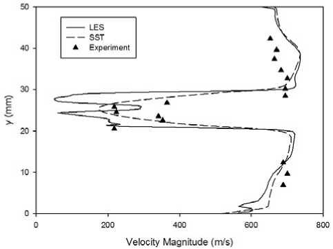
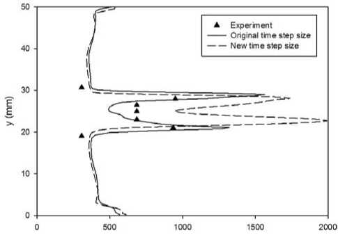
Figure 2. Comparisons of velocity under two turbulence models (x=78mm)

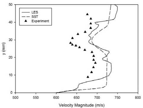
Figure 3. Comparisons of velocity under two turbulences (x=207mm)

Discussions give the general theory illustration of relation between turbulence model and numerical results in the combustion comber, but not enough to the vivid explain the rules. In this section, the authors give two velocity comparison figures (Fig.2 and Fig.3) under two models at different positions, which the x-components are 78 mm and 207 mm, respectively. It is clear that: (1). The two numerical results of the flow field, which near the wedge-shaped flame holder, agree well with the experiment data through comparison and this conclusion for the upstream is invalid for the downstream. This is agreed with the existing findings [15]; (2). The differences between the two numerical results are middle region in the near field and underside part in the far region. There are three main reasons that can account for the phenomena in practice. The first one is that any slight differences in the upstream area can lead to a significant difference in lower reaches. The second one mentioned is the results of the downstream region are influenced by the simplified hydrogen kinetic model. The last one is there is a hairlike discrepancy in the position between computation model and tester. This is also important to match condition between the calculated and measured values, and the nuance, more or less, have relationships to the outputs. In addition, Boubier’s studies showed that: Reynolds-Averaged Navier-Stokes (RANS) can be only used in the preliminary analysis on the combustion performance. LES, which considered the precise of time and large-scale space, is approximate to analyses of combustion and the accuracy is not ideal [16-19].

О             500            1000           1500           2000

Static temperature (К)

Figure 4. Comparisons of temperature under two turbulence models (x=78mm)

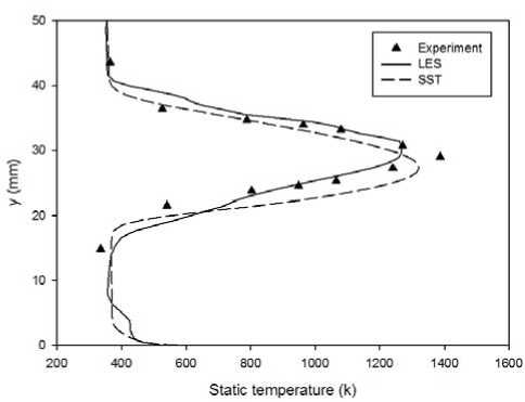
Figure 5. Comparisons of temperature under two turbulence models (x=207mm)

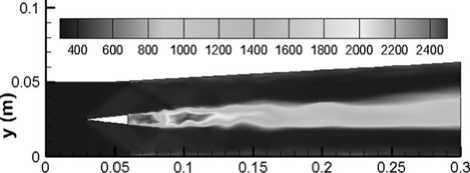
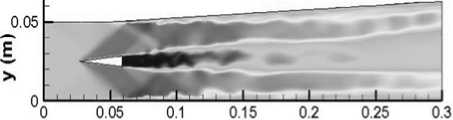
The temperature distribution within the ramjet chamber plays an important role in performance parameters of ramjet. The Fig.4 and Fig.5 give the temperature contrast under the same calculation condition. It does can be seen that the SST is not accurate enough for calculating temperature of the Y-axis middle region. However, the LES is the most properly used for computing the parameters both in the near and far field. In addition, it is also shown the high-temperature region in shear layer of downstream is coincident with the value measured by Yang [20], which shown in Fig. 6.

x (m)

Figure 6. Static temperature contour under LES model (K)

The burning of ramjet is a complex combustion, and the other mode is the cold flow. Considering the characteristic and the different between the states of these two operating conditions, this paper selects four positions ， which the x-components are 78 mm, 125 mm, 157 mm and 233 mm respectively and gives the four velocity comparison figures, which are given in Fig.7 to Fig.10, under two turbulence models to give a vivid illustration of this working mode. The results of the numerical calculations and experimentations point out that: (1).When the turbulence model is LES and the x-components equal to 78 mm, there are same errors in the midcontinental region of Y-axis, but the two simulation results are both in good agreement with experimental data at another position; (2). The differences of the numerical results are not significant at the same position of x-axis except the middle of Y-axis coordinates where the SST provides more accurate; (3). The LES calculated values shows a slight oscillation in some areas, but this is not appeared in other models.

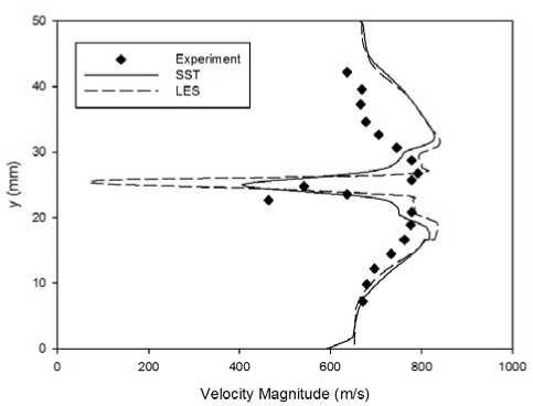
Figure 7. Comparisons of velocity of cold flow condition under two turbulence models (x=78mm)

As mentioned previously, the cold flow model was different with combustion conditions. So the pressure distribution is another validation parameter, which chosen by the authors. Fig. 11 gives the static pressure contrast curves at the Y-components is 25 mm, which is half the height of the calculation model, under the uniform operating conditions like that mentioned above paragraphs. From the figure, it can be known that: (1). Two numerical results exist remarkably different in the wedge-shaped flame holder areas; (2). During areas which after the holder, the two outputs both agree with experiment results well except for a few positions.

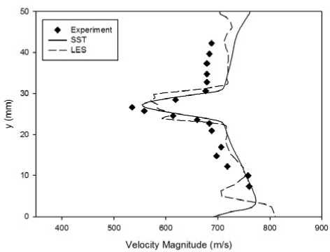
Figure 8. Comparisons of velocity of cold flow condition under two turbulence models (x=125mm)

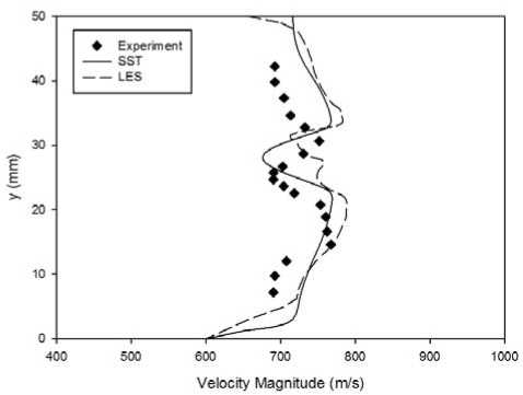
Figure 9. Comparisons of velocity of cold flow condition under two turbulence models (x=157mm)

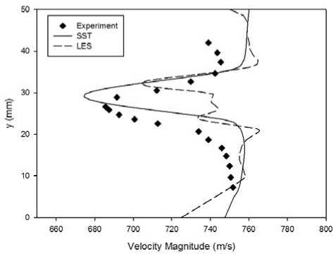
Figure 10. Comparisons of velocity of cold flow condition under two turbulence models (x=233mm)

In summary, the LES is shown to be capturing important flow features and making accurate predictions of main parameters such as velocity and static pressure, etc. at most positions. Therefore, this model is the proper choice for attaining reality data as possible.

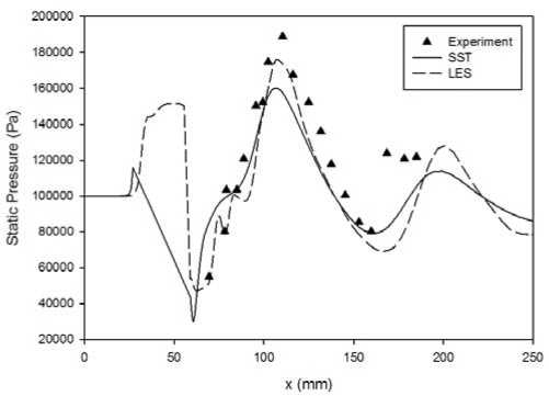
Figure 11. Comparisons of static pressure of cold flow condition under two turbulence models (y=25mm)

• B.    Time Step Size

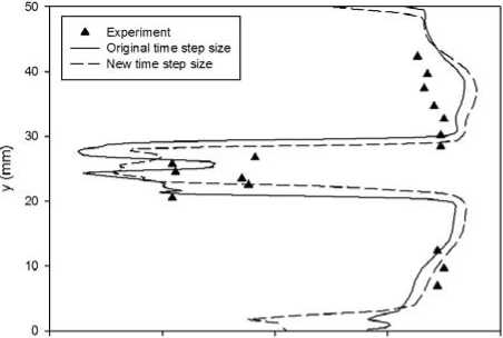
It is common faced the critical selection of time step size in numerical simulation when the turbulence model is LES. Moreover, the fluid analysis often cannot continue to study because of serious errors, which causes by the wrong choice of that parameter. Two choices of time step size are chosen to be used in the calculation in order to verify the analysis of the combustion condition. One is the original setting in the previous section, and the value is 1.0×10 ^-6 second, which is selected based on many reasons, such as meshes characteristics, intake parameters, experiences, etc. and the other is the 1.0×10 ^-5 second. The following two figures (Fig.12~13) give the velocity comparison of the positions, which the x-components are 78 mm and 207 mm, respectively. From those figures, we can come to the conclusion that: (1). At the x-axis equal to 78 mm, there is the inconspicuous difference between two groups of numerical values, which agree with the experiment, except for a few positions; (2). The velocity values gained under those time step sizes are quite distinct between the CFD and experimentation data. However, calculative results approached to experimental values of the conditions for which the time step size is original setting, and the advantage is appeared as compared with the new size.

О              200             400             600             800

Velocity Magnitude (m/s)

Figure 12. Comparisons of velocity of different time step size (x=78mm)

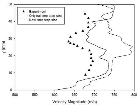
Figure 13. Comparisons of velocity of different time step size (x=207mm)

Static Temperature (К)

Figure 14. Comparisons of temperature of different time step size (x=78mm)

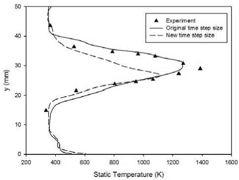
Figure 15. Comparisons of temperature of different time step size (x=207mm)

Figure 14 and Fig. 15 gave the temperature distributing under those two settings at the same positions. It can be known that: (1). There is a significant oscillation within the main combustion region under the new time step size at the x-component is 78 mm, and this is obviously not in line with the original numerical results and experimental values; (2). To some extent, these settings have brought a greater degree of precision to the authenticity of flow field in a partial area of the far-field region. However, there is still some difference within the region, where the values of Y-component vary in the range from about 27 mm to 40 mm.

To illuminate these rules, the authors give the temperature contours in the symmetry plane under new time step size. The figure shows that: although the high-temperature region is appearing near the x-component equal to 78 mm, there are some major differences between temperature distribution and the existing findings.

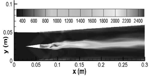
Figure 16. Static temperature contour under new time step size (K)

To conclude, the result of new setting not agreed well with the existing results under the combustion condition, so the cold condition is not necessary to be discussed. In addition, those conclusions also indicated the rightness of the original time step size and the reliability of this computing method, which is selected by the authors in this paper.

• C.    Mesh

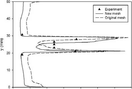
  Considering the complexity of the flow within a ramjet combustion chamber, involving compressible flow, shock, turbulent and combustion, have led to increasing reliance on mesh quality as the key to gain credible data from the numerical computation. To analyze the influences of this factor, the authors adopt two representative meshes, namely, the primary mesh and modification mesh, whose number of cells in the computational domain decreased from 810900 to 432800, and the analysis is carried out for the precision of the computing meshes by comparing two results of calculation in the same initial condition. The authors give the following figures (Fig.17~18) of velocity comparison at the x- coordinates are 78 mm and 207 mm respectively under two meshes. From the calculated and experimental values, it has been discovered that in the upstream region, there is some oscillation and error appear within the Y-component range from 20 mm to 30 mm under two meshes condition, and the oscillation amplitude of primary mesh is larger than the modification one. In addition, the calculative results at other locations agree with observed ones very well. Results from CFD and test study also showed the computational accuracy of the new mesh is higher in far-field velocity forest than the other one, but the two meshes both have certain extent limits and shortages in achieve real distribution of the velocity in detail.

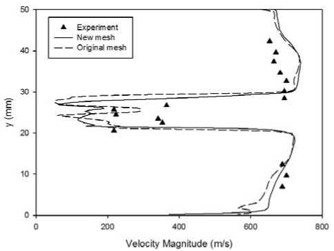
Figure 17. Comparisons of velocity of different mesh (x=78mm)

Figure 18. Comparisons of velocity of different mesh (x=207mm)

Similarly, detailed analysis of these meshes is based on the temperature. Fig. 19 and Fig. 20 depicted this parameter distributing of the same positions, which are mentioned in above paragraphs. It’s can be seen in those figures that: (1). The calculated results of the primary mesh are in good agreement with the experimental data both in the near-field and far-field region; (2). Although the error, which is between simulation results under the new mesh and experiment data, are smaller in the upstream and part positions of downstream, the computation values of the Y-axis middle region not agreed well with the measured values.

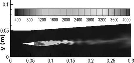
In order to validate the rules between mesh and temperature, the a static temperature contour on the symmetry plane under new mesh case, as shown in Fig. 21 is made to see how well the method fits the given combustion chamber. It can be observed that: (1).There is a significant difference between two distributions under different meshes; (2).The abnormal high-temperature zones, where the values of x-component vary in the range from about 50 mm to 160 mm, are appeared and a few temperatures during these areas are above 4000 K. These are totally at variance with the existing theory and conclusions. Thus, it could be concluded the new mesh is improper in this numerical simulation. there is no need to verify the cold condition.

The numerical tests are designed to understand the actual state of the ramjet combustion chamber. While the scope of above discusses and taking into account the combustion mainly occurs in the near-field zone, it could be concluded the method which used by this paper is appropriate, and computing results are accepted as an authentic data.

200      400      600      800     1000     1200     1400     1600

Static temperature (К)

Figure 19. Comparisons of temperature of different mesh (x=78mm)

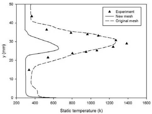
Figure 20. Comparisons of temperature of different mesh (x=207mm)

x (m)

Figure 21. Static temperature contour of new mesh (K)

• III.    Noise Prediction

It is well accepted the flow, mixing, combustion of gases with high-temperature and high-speed within the ramjet combustion chamber contribute to noise, but their main component is essentially aerodynamic noise, which is caused by the turbulence. That is to say, the character of noise field is determined by the turbulence essence,

and its principle can be adequately described with the

Lighthill acoustic analogy equation. This is represented

by the following equation [21]:

∂ ² ρ ∂ t²

c ₀ 2 _∇ 2 ρ ₌

∂τij ∂xi∂xj

Where ρ is density, c₀ is sound speed of homogeneous medium and τ ij is stress tensor.

main factors which may account for this phenomenon can be summarized as follows: the first one is hydrogen ejects into the chamber with high-speed; the second one is the hydrogen react vigorously with the oxygen in the air; the last one mentioned is the influences of LES and boundary-layer are obvious gradually with increasing x-coordinates.

According to above analysis, in combination with well characteristic of computational model, 21 observation points are selected. Their coordinates, which are arranged into three lines, are listed in Table.6 [21].

TABLE 5 FWH METHOD PARAMETER

Parameter	ρ(kg/m3)	V a (m/s)	P 0 (Pa)
Value	1.225	340	2×10-5

Where ρ and Va are density and sound speed of far-field respectively, P0 is the reference acoustic pressure.

The other need to be mentioned is selecting the observation point, which is also marked as the receiver in this paper, to obtain the exact distribution of noise field, and its selection should be based on flow characteristics. Because the correctness and precision of calculation method have been tested and verified in the previous section, and then it is reasonable and feasible to use its results to choose the coordinates of observing points. The following two figures (Fig.22 and Fig.23) give contours of dynamic pressure and Mach number on the symmetry plane, respectively.

TABLE 6 RECEIVERS POSITIONS

Number	Coordinate
	x (mm)	y(mm)	z(mm)
1	0.00	50.00	22.50
2	27.70	50.00	22.50
3	59.00	50.00	22.50
4	121.87	53.77	22.50
5	169.18	56.25	22.50
6	235.18	59.70	22.50
7	300.00	63.10	22.50
8	0.00	50.00	45.00
9	27.70	50.00	45.00
10	59.00	50.00	45.00
11	121.87	53.77	45.00
12	169.18	56.25	45.00
13	235.18	59.70	45.00
14	300.00	63.10	45.00
15	0.00	0.00	22.50
16	27.70	0.00	22.50
17	59.00	0.00	22.50
18	121.87	0.00	22.50
19	169.18	0.00	22.50
20	235.18	0.00	22.50
21	300.00	0.00	22.50

As mentioned previously, there were two different conditions, namely, combustion and cold flow, the analysis is carried out for the likenesses and differences of this by comparing the distributing of noise in the same initial condition separately in next paragraphs.

20000 100000 180000 220000 260000 300000 340000

x(m)

Figure 22. Dynamic pressure contour on the symmetry plane (Pa)

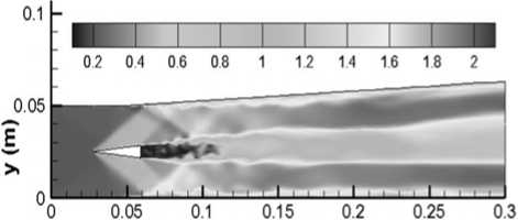
Figure 23. Mach number contour on the symmetry plane

A. Combustion Condition

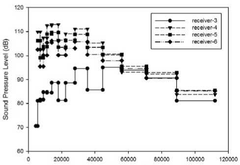
1/3-Octave Band (Hz)

Figure 24. Spectrums of 1/3-Octave Band (receiver 3~6)

The results indicate that the parameter distribution of regions, which near the Hydrogen inlet is uniform, but this uniformity is destroyed in the downstream zone. The

It has become known that though detecting real-time acoustic pressures of every point and its corresponding

changes, we can calculate the frequency and other parameters of field noise. Figure 24 gives four points’ relationship between the 1/3-octave band and sound pressure level (SPL). From this figure, we can conclude that: (1). There are a few differences between the three receivers, whose serial numbers are 4, 5 and 6, respectively. The maximum value of each point is also gained at the frequency of about 18000 Hz. In addition, their SPL is all above 90dB at the low frequency and then, it is decreasing as 1/3-octave band increases; (2). SPL of receiver-3 is significantly lower than the other three positions, but the difference is decreased with increasing frequency. The main reasons are the wedge-shaped flame holder is selected as the sound source and that point located in the tail area.

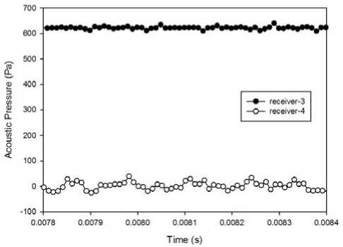
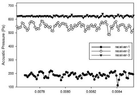
Figure 25. Sound pressure vs. time (receiver 3~4)

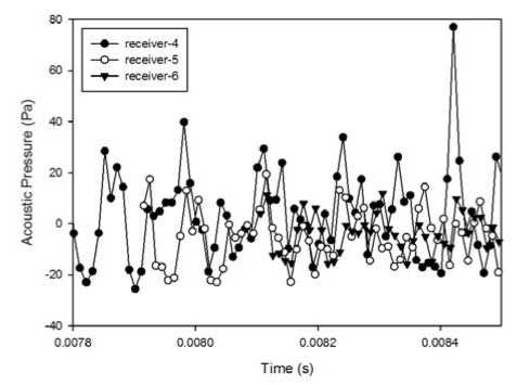
Figure 26. Sound pressure vs. time (receiver 4~6)

Because of results showed there are obvious discrepancies of SPL between the receiver-3 and another three points, Fig. 25 and Fig. 26 depict the timedependent curves of sound pressure of receiver 3~4 and 4~6, respectively. It’s can be seen in those figures: (1). The receipt times of the receiver-3 and receiver-4 show a little difference, and the D-value is 0.1628 ms because the distance between them is short, and the sound source is the wedge-shaped flame holder. However, there are significant differences in sound pressure of these two observation points and the mean values during calculating time are 622.690 Pa and 3.528 Pa, respectively; (2).The mean values of receiver 4~6 are similar, and these observation points have received flow information in turn at computing time are 7.7815 ms, 7.9154 ms, 8.1064 ms, separately; (3). In several points, the maximum difference value between the receiver-4 to receiver-6 is about 60-70 Pa, which is far less than corresponding sound pressure of receiver-3. All of those demonstrated the correctness of above analysis in the previous paragraph.

In accordance with the supersonic noise theory, noise consists of three basic components, namely turbulent mixing noise, broadband shock noise and whistler-type noise. It is known well enough the first part is an occupied leading place in downstream, and the second one is dominated in upstream. In addition, the third one diffused from the lower reaches to the upper course. To illuminate the differences between the three receivers, which located in upstream, the Fig. 27 shows the variation of sound pressure with time. From this figure, the authors can come to the conclusion that: (1). The differences of receipt times of these observing points are inconspicuous, and the maximum D-value is only 0.0667 ms.The reason is the distances of x-direction between them is short; (2). Evidently, there are dissimilar in the sound pressure values due to the wedge-shaped flame holder is chosen as the sound source. The pressure data change with the time indistinctly, and the decrease degree increased with x-coordinate decreased.

Time (s)

Figure 27. Sound pressure vs. time (receiver 1~3)

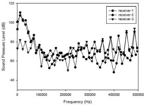
Figure 28. Sound pressure level vs. frequency (receiver 1~3)

Figure 28 further gives the relationships of those three receivers between the SPL and frequency. It is clear that there are not significant differences in SPL except the portion region, and the values of low frequency are greater than that of high ones.

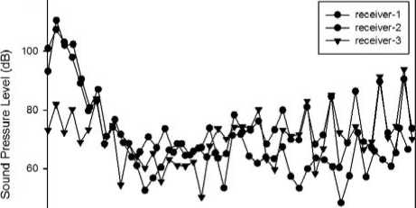
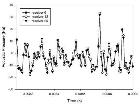
Figure 31. Sound pressure vs. time(x=235mm)

0         100000       200000       300000       400000       500000

Frequency(Hz)

Figure 29. Sound pressure vs. time (x=59mm)

Next, Fig. 29 shows the three change curves of the sound pressure as a function of time at x-coordinate equal to 59 mm, it is considered that: (1). Receipt times of three receivers are identical because they are equidistant from the sound source;(2). The sound pressures kept stabilizing during computing time, and the mean values are 622.690 Pa, 610.734 Pa and 685.287 Pa, respectively. In addition, Considering the value of the receiver-3 is a benchmark, the relative error of receiver-10 is 1.920% and the corresponding value of receiver-17 is 10.053%.These conclusions also explain the sound pressures of lower side is greater than that of upside at x-direction value is 59 mm.

To analyses pressure laws of upstream, the Fig. 30 gives the relative errors of receiver-8 and receiver-15 selecting SPL of receiver-1 as a datum mark. The results indicated the values of upside are less than that of the underside, but not as obvious as that of locations, whose x-coordinate is 59 mm. Furthermore, the authors drew a uniform conclusion from the Fig. 31, which depicts the time-dependent curves of sound pressure at x-direction equal to 235 mm.

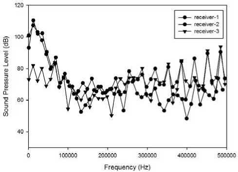
Figure 30. Δap vs. time (x=59mm)

B. Cold Flow

As mentioned previously, the clod flow was the other important working mode. To understand this condition better, the authors not only analyses the variation of different positions, but also comparing the likenesses and dissimilarities between these two conditions, so the relationships of receiver-3 and receiver-4 between acoustic's pressures and time are shown in Fig. 32. And the authors conducted that: (1). Receipt times of two receivers are not notable, and the difference is only 0.16289 ms. The change law is found to be similar with results of the combustion condition; (2).The sound pressures kept stabilizing during computing time, and the mean values are 608.99 Pa and -163.69 Pa, respectively. Compared with the combustion condition, the sound pressure of receiver-4 is significant difference, but this rule does not apply to receiver-3 as given in Fig. 33.

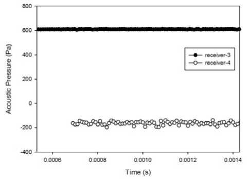
Figure 32. Sound pressure vs. time (receiver 3~4)

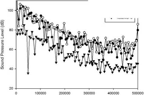
After carrying on fast Fourier transform (FFT) on acoustic pressures at these observation points, the two change curves of the sound pressure levels as a function of frequency are shown in Fig. 34. It can be seen the value of receiver-4 is higher than that of the receiver-3, and the maximum D-value is 25 dB. In addition, the research also makes it clear that sound pressure levels of two observation points markedly decrease with increasing frequency, and the change rules are alike.

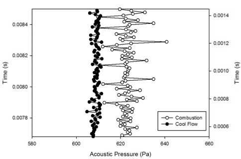
Figure 33. comparisons of acoustic pressure between combustion and cool flow (receiver-3)

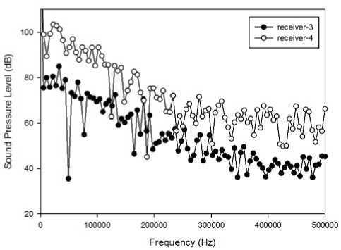
Figure 34. Sound pressure level vs. frequency (receiver 3~4)

Similar to combustion condition, at the conditions for which the computing settings is the same, i.e. time step size is 1.0×10 ^-6 second, the acoustic pressure changing with time at the receiver-4 to receiver-6 are shown in Fig. 35, to analyses the noise distribution of lower reaches. We can see the receivers received information in turn according to the flow direction and positions of observation points. The time interval of receiver-4 and receiver-5, receiver-5 and receiver-6 are 0.13383 ms and 0.19103 ms, respectively. These results verified well with conclusions of the previous section.

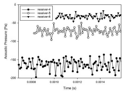
Figure 35. Sound pressure vs. time (receiver 4~6)

However, compared with the combustion condition, differences of the mean values of sound pressures are increased during the calculating time. To explain the conclusion further, Fig. 36 gives the receiver-6’s relationships between sound pressure and time under two kinds of conditions.

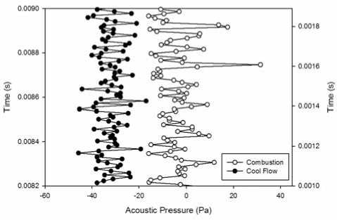
Figure 36. comparisons of acoustic pressure between combustion and cool flow (receiver-6)

After carrying on FFT on acoustic pressures at these observation points, the relation between SPL and frequency has been studied, which are shown in Fig.37. It can be seen that their variations of the SPL with time are similar, and the mean values of sound pressures are 72.25 dB, 68.65 dB and 64.58 dB, respectively.

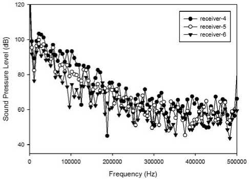
Figure 37. Sound pressure level vs. frequency (receiver 4~6)

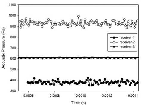
Figure 38. Sound pressure vs. time (receiver 1~3)

The variations of sound pressure of upstream observation points are given in Fig.38, in order to analyze the noise field in detail. We could see that there are a few differences in receive time, and the interval is only 0.00426 ms because distance between the receiver-2 and receiver-3 is short. This looks like that in combustion condition.

As shown in Fig. 39, the law of mean values of sound pressure is different under two conditions. The decrease trend of receiver-2 not only cannot be found, but the value mounted into 927.84 Pa. Those who need a specification are that there is a certain error at upstream zone when the turbulence model is LES under the cold flow, and it will most likely affect the calculated authenticity, in one-way or another. In addition, time change rules under two conditions are same. However, the mean value of sound pressure under cold flow is 379.82 Pa, and the value is improved about 50.54% compared with the combustion.

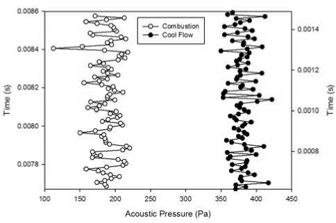
Figure 39. comparisons of acoustic pressure between combustion and cool flow (receiver-1)

• ■ receiver-1

—O— receiver-2

V receiver-3

Frequency (Hz)

Figure 40. Sound pressure level vs. frequency (receiver 1~3)

Then, the relations of three observing points between SPL and frequency have been shown in Fig. 40. A few results are gotten as bellow: (1). Variations of these receivers are similar, and the SPL value decreases with increasing of the frequency; (2).The mean values of the receiver-1 and receiver-2 are 72.49 dB and 76.07 dB, respectively, and they are both greater than that of receiver-3, which value is 54.12 dB. It indicated the SPL is being increased during propagation upward. This conclusion does not match with the combustion conditions.

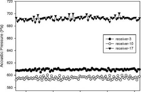
The three receivers, whose x-coordinate are 59 mm, are selected to research noise distribution at the same location and the rules of sound pressure with time are given in Fig. 41. We may safely draw the conclusion that: (1).The receiving times of these observation points are the identical because their x-direction values are all uniform;(2).The sound pressures kept stabilizing during computing time, but their mean values are the definite differences, and the values are 608.99 Pa,595.15Pa and 692.37 Pa, respectively. It means the differences between receiver-3 and receiver-10, which are located on the upward side, are little and their sound pressures are lower than that of the underside. The result coincides with that of the combustion condition.

0.0006        0.0008        0.0010        0.0012        0.0014

Time (s)

Figure 41. Sound pressure vs. time (x=59mm)

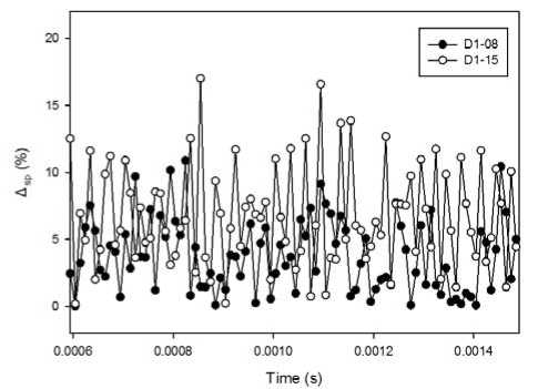
Figure 42. Δ ap vs. time (x=59mm)

In order to give an intuitionist relationship, assuming the data of receiver-1 is a benchmark, Fig. 42 gives the relative errors of receiver-8 and receiver-15. We could see there is no marked sound pressure difference between the upside points, and the average error is about 3.48%. In addition, the corresponding data of the underside receiver increase slightly and the mean value can reach 6.60%. However, it is still lower than 13.69%, which is gained at x-coordinate equal to 59 mm.

The relations of downstream receivers between sound pressure and frequency have been shown in Fig. 43, and the results have further validated the conclusions, which have been referred above, are correct.

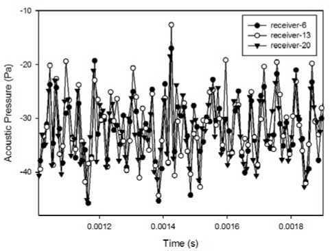
Figure 43. Sound pressure vs. time(x=235mm)

• VI. Conclusion

Based on flow verification and noise prediction under the combustion and cold flow, the results are shown that:

• 1) .The method which is used in this paper can be used to accurate calculate the complex flow parameters in the combustion chamber;

• 2) . On the premise of the flame holder is the sound source, dominant frequencies are concentrated at the higher-frequency band under the combustion and cold flow conditions. Moreover, the rules of the sound pressure with x-coordinate, which is located in upstream or downstream, are obviously different;

• 3) .Noise laws are identical with the same horizontal position under the combustion and cold flow conditions.