Computing Method and Hardware Circuit Implementation of Neural Network on Finite Element Analysis

Author: Likun Cui, Wei Wang, Zhuo Li
Journal: International Journal of Intelligent Systems and Applications(IJISA) @ijisa
Article in issue: 5 vol.3, 2011.
Free access
The finite element analysis in theory of elasticity is corresponded to the quadratic programming with equality constraint, which can be further transformed into the unconstrained optimization. In the paper, the neural network of finite element solving was obtained on the basis of Hopfield neural network that was reformed. And the no error solving of finite element neural net computation was realized in theory. And a design method to construct an artificial neuron by using electronic devices such as operational amplifier, digital controlled potentiometer and so on was presented. A programmable hardware neural network of finite element can be build up by using analog switches to interconnect inputs/outputs of hardware neurons. The weights, biases and connection in the hardware neural network of finite element can be adjusted automatically by microprocessor according to the results of train to controlling system, This programmable hardware neural network of finite element has some more adaptability for different systems. In addition, the authors present the computer simulation and analogue circuit experiment to verify this method. The results are revealed that: 1) The results of improved Hopfield neural network are reliable and accuracy; 2) The improved Hopfield neural network model has an advantage on circuit realization and the computing time, which is unrelated with complexity of the structure, is constant. It is practical significance for the research and calculation.
Finite element method, Hopfield neural network, analogue circuit, simulation, operational amplifier, digital controlled potentiometer
Short address: https://sciup.org/15010223
IDR: 15010223
Text of the scientific article Computing Method and Hardware Circuit Implementation of Neural Network on Finite Element Analysis
Published Online August 2011 in MECS
With the rapid development of computer software and hardware technology, finite element method has been widely applied to the structure analysis and design. It is very slow to deal with large-scale and complex engineering structure and the efficiency is low because the traditional calculation program for structure optimization is based on all serial algorithms in a single computer [1]. And the contradiction between the large computes scale and low computational ability becomes more and more urgent, so the parallel computing method has important meaning for finite element method. However, common methods cannot create enough computational efficiency needed in practice [2].
The neural network is a large-scale nonlinear dynamics' system, and it has own characters, such as high parallel processing ability, strong robustness, fault-tolerance, learning ability and adaptability, and shows to superiority in setting up model for complicated system, so it is suited for many aspects in industry and profession. In addition, the neural network is considered as a dynamic circuit, and it can be used for high-speed parallel computation and is easy to attain the solutions within the time constant [3]. So, the finite element analysis in theory of elasticity is solved by modified Hopfield neural network and verified by the computer simulation and analogue circuit experiment in the paper. The article also provides a design method to construct an artificial neuron in theory by using electronic devices such as operational amplifier, digital controlled potentiometer, analogy switch and so on. A programmable hardware neuron networks can be built up by using analog switches to interconnect inputs/outputs of hardware neurons. The weights, biases, activation functions and connection in the hardware neuron networks can be adjusted automatically by microprocessor according to the results of train to controlling system. This programmable hardware neuron networks has some more adaptability for different systems.
-
II. Elasticity Finite Elements Model Using Improved Hopfield Neural Network
The finite element analysis in theory of elasticity is corresponded to the quadratic programming with equality constraint, which can be further transformed into the unconstrained optimization and the Hopfield neural network is a good method in the field of optimization calculation, so that problem can be solved by this method. Beside this, the previous work on neural network has indicated that the potential energy functional equals to the objective function of the finite element method and the maximum or minimum point, which is the stable equilibrium point of the network system, is the solution.
-
■ A. Quadratic Optimal Method for Elasticity Theory Problems
It is well known that system optimization is the nature of computation. In this section, a detail explanation is proposed for this point in the context of elasticity [4].
-
1) Equilibrium Equation
-
7, = 0 ( i =1,2,3, V e V ) (1)
Where оу j is stress and f is volume force.
-
2) Geometrical Equation
E j = J j u ji )
( i , j =1,2,3, V e V )
Where E j is strain and u i j is displacement.
-
3) Physics Equation
^j = DyE(i,j,k,1 = W, V e V)
Where Dijkl is elastic constant
-
4) Boundary Condition
T = T (i =1,2,3, S e Sff)
ui = ui (i=1,2,3, S e Su)
Where T is area force, S CT is force boundary and S u is displacement boundary.
According to the principle of the minimum potential energy, elastomer under external force is balanceable and the total potential energy is given by:
П , = J V (2 D (W s,s„ - fu i ) dV - J S . TudS (6)
Equation (6) depicts the equilibrium equation and force boundary of elastic body and its minimum value is true solution in all possible displacement field , which is meet the conditions (2) and (5). This means that the finite element analysis in theory of elasticity can be transformed into the optimization problems under an equality constraint condition. The mathematical model is given by:
min П p = J V ( 2 Dva £ v£a - fu, ) dV - J S TudS
/ 2 E = ( j u^) (V e V) (7)
■ [ u, = u, (S e S )
ii u
The authors divided continuum into m elements (including m1 force boundary element, n nodes and n1 displacement boundary nodes) by finite element with respect to mathematical model transformation [5].The new mathematical model is given by:
min П (5 )=- 5 T K 5 - f T 5
-
< _ 2_ (8)
_ s . t A 5 = 5 ( S e S u )
Where K is global stiffness and its value is m
K = ^ j BTDBdV, f is node load array and its value is mm1
f = ZJ, ( N T f ) dV + EL ( N T T ) dS , T is
-
e = 1 V e e = 1 S ^ e
surface force, 5 is node displacement array, A is constrained matrix, B is strain matrix, D is elasticity matrix and N is shape function matrix.
The above optimization problem is equivalent to the following linear equation [6]:
K 5 = f (9)
Where 5 x is equal to 5 i ( i = 1,2, l , s ) .
For static problem, compulsory boundary conditions are directly substituted into (9) and the new equation is given by:
K ' 5 ' = f ' (10)
Where K is positive definite matrix .
Finally, (8) is transformed into the following unconstrained optimization problem and its solution is confirmed when K is the positive definite matrix according to the optimization theory.
min П ' ( 5 ' )=2 5 ' T K '5 ' - f T 5 ' (11)
-
■ B. Improved Hopfield Neural Network
The previous work has indicated that the energy functional of neural network equals to the objective function of the finite element method, so its mathematical form, Lyapunov form [7-9], and dynamic equation are given by (12), (13) and (14):
E=V( ^ )=2 5 T K 5- f^5 (12)
E - " 2 5 T W 5 - [ b T - (,''- L -1)] ^ (13)
d5 „.
г--= -Кб+ / dt
5' (0) = p
Where W is equal to — K and
R 1 , 1 / R 2 ,..., 1 / R r )of potentiometer resistance is used to represent the weight of input signal, the product ( u j /R j ) of the input signal and its weight is input current flow of operational amplifiers, then, The mathematical model is given by:
f T is [bT — (1,1, l ,1)] .In addition, stability of this network is discussed by:
dE л ! д \ ddd' s^ did
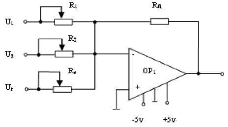
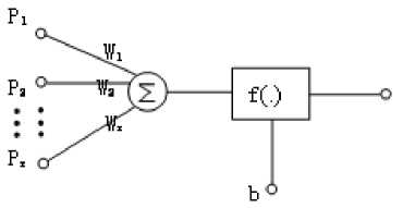
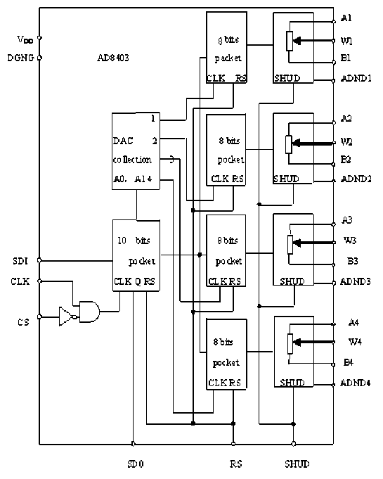
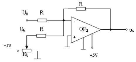
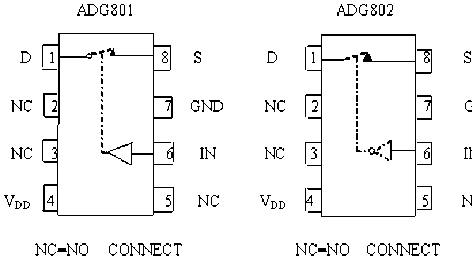
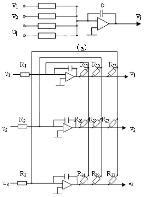
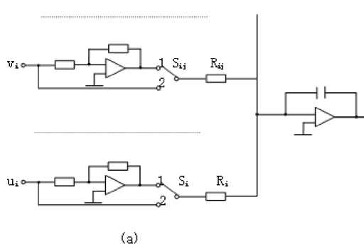
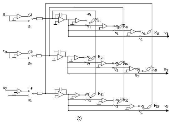
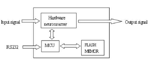
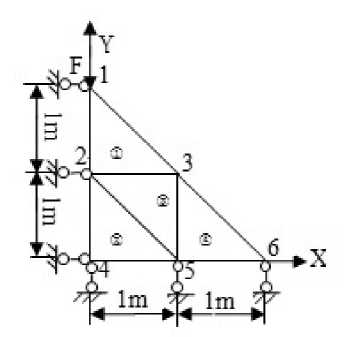
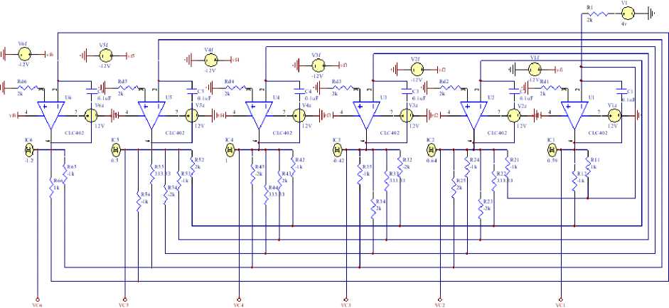
= — £[ ]' =—^У( -)2 According above theory, the diagram of improved Hopfield neural network is proposed in fig.1: uu u u- =- Rf,(R;+R;+L+R^) (l8) To achieve automatic adjustment of neuron input signal weights, the potentiometer R1 R2,... , Rr in fig.3 can be digital potentiometer AD8403. The principle chart of the internal structure of AD8403 is shown by fig. 4. Fig. 1 Diagram of improved Hopfield neural network III. NEURAL NETWORK HARDWARE IMPLEMENTATION ■ A. Neurons Hardware Implementation Neurons are basic processing units of artificial neural network. It is usually a non-linear element has many inputs but only single output. A typical neural model is shown in fig.2. Its input/output relationship is given by (16): a = f (£ ®jPj+ b) (16) j=1 Its matrix form is A = f (W x P + b) (17) Fig. 3 Neuronal input weighted summation circuit Fig. 2 Single neural model ■ B. circuit of the signal weight sum For neural model in fig.2, its input signal weighted summation parts are realized by the hardware circuit showed in fig.3. Operational amplifier OP1 is connected into adder form. The input signal u1, u2, …, ur are supposed as the standard output voltage signal (- 5V - + 5V) of various signal sensors, hence, the reciprocal (1 / Fig. 4 Internal structure principle diagram of digital potentiometer AD8403 It consists of four independent potentiometers. The resistances (norminal value) between the fixed ends of potentiometers generally have four specifications: 1KΩ, 10KΩ,50K Ω and 100K Ω. Each potentiometer has two fixed ends (A and B) and one sliding contact (W), the resistance between W end and B end is decided by the datas is placed in its serial input registers, and there are 256 branch decision points. The biggest characteristic of digital potentiometer is its programmable ability, so it also is called numerical control variable resistor. Under the action of the clock CLK, 10 bits serial datas are placed in through serial data input terminals SDI. The 10 bits datas formats are D7 D6 D5, A1 A0 D4 D3 D2 D1 D0. If sliding arm W and A is connected, the variable resistor RWB computation formula is: Rwb (Dx) = (Dx )/256 x R^b + Rw If sliding arm W and B is connected, the variable resistor RWA computation formula is: Rwa (Dx) = (256 - Dx) /256 x Rab + Rw ■ C. circuit of Deviation comparison Considering the role of deviation b, the comparison of ub and u0 can be realized by the deviation compared circuit shown in fig.5 (potentiometer Rb shown in figure is also digital potentiometer AD8403). In fig.5 circuit, input resistance value is equal with the feedback resistance valve (both are R), the deviation ub is positive voltage, and u0 is inverse with the input signal through former treatment of the OP1 operational amplifier. Therefore, D-valve of u0 and ub is a signal inputted amplifier OP2 in practice. The comparison between them was realized. In addition, the operational amplifier OP2 which uses single polarity power (+ 5V) has output only when the signal u0 is bigger than deviation ub. Fig. 5 Circuit of Deviation comparison The mathematical model is given by: Ux =-(u0 + ub ) After two reversed-phase operations of operational amplifier OP1 and OP2, ux is changed into same phase with u1, u2,... ur. ■ D. connection circuit between inputs and outputs The analog switch ADG801/802[10] is chosen to control circuit for the automatic connection realization of different input and output signals between neurons. The diagram of ADG801/802 analog switch pins is shown as fig.6. It is supplied power by1.8-5.5V single power. The largest conduction resistance is less than 0.4 Ω, conduction resistance flatness is 0.1 Ω; Switch hige current capacity of is 400mA; Double guide conduction; Response time is 35ns; Low power consumption; TTL/CMOS compatible input; Analog switch ADG801 is often open (IN = 0 disconnect, when IN = 1 conduction), ADG802 is often closed (IN = 1 disconnect, when IN = 0 conduction). Fig. 6 Schemes of analog switch pins In addition to the above analog switches, there are ADG706, ADG707 etc. IV. NEURAL NETWORK HARDWARE IMPLEMENT ON FINITE ELEMENT According above theories, the Hopfield model circuit can be changed into the form in fig.7, notably the neural network is a linear system. (b) Fig.7 The network structure of finite element neurons and three nodes network The circuit shown by following equation. fig.7 can be described in dv (t) m 1 u c —- = -> —v, - L dt ^x R„ j R ij i uo - Rf Because By comparison with expression (15), we find they are equivalent and meet the following relations: T ij c = s (20) 1 " — = ku Rij ij (21) ui- = - f Ri i (22) v, = a; (23) Rij kij can be positive, negative or zero, also can be positive, negative or infinite. An invert and vR on-off switch can be set between j and ij in order to solve this problem. And i also can be disposed in this method. The circuit is shown in fig.8(a) after disposal. In different finite element solution, the matrix K, F is different. In order to realize generality of the neural network in solving the finite element problem, resistance R must be variable resistor and u be set for a constant. A neural network solving system can only solve the finite element solving problems whose matrix is n×n. In order to solve the problems whose matrix is under n×n, inputs and outputs between neurons be controlled by switches. And so, neural network circuit shown in fig.8 (a) must be changed into the form shown in fig.8(b). Fig.8 Corresponding circuit diagram Finite element neurons and three nodes network According to the hardware neural model realization method has been discussed in the previous text, the variable resistors and switches in the circuit shown in fig.8 must be respectively digital potentiometer AD8403 and analog switch ADG801 or ADG8. The hardware neural network system structure chart is illustrated by fig.9. Fig.9 The structure schematic drawing of hardware neural network system The System consists of a hardware neurons array (containing a number of neurons hardware circuits), several analog switches, a non-volatile storage (such as Flash memory), a microcontroller and relevant interface circuits. All digital potentiometers and analog switches have their separate addresses in the system board.The weights, thresholds, input/output connections are controlled by MCU based on digital potentiometers, analog switches for programming setting (adjustment). As shown is fig.2, consider a sheet with thickness t=0.1mm, elastic modulus E and Poisson's ratio μ=0.3 subject to force F=10KN. Find the displacement of each point assuming the gravitation is zero. Fig. 10 Structure schematic diagram the authors use the following three different initial input values, which are mutually orthogonal vector. д1 (0) = ( 0.59 0.64 -0.42 1 00 д2 (0) = ( 0.77 0.32 -0.57 0 10 д3 (0) = ( 0.20 -0.68 0.76 0 0 Table I lists the results of network circuit and theoretical values and the unit of all the circuit outputs in the following tables are N.mm.E-1. It can be observed that circuit simulation solutions under three initial input values are same and the difference is small between the simulation and theoretical value. This is because the influence of input offsets like voltage and electricity. In order to find the displacement of each point, the boundary conditions are introduced to the calculation domain. The global stiffness matrix is modified, and the following expression is results: In order to make the calculated result is universal, TABLE I The Results of Network Circuit and Theory Outpu t V1 V2 U3 V3 U5 U6 Case 1 -3.257 -1.256 -0.0932 6 -0.377 0 0.164 4 0.154 6 Case 2 -3.257 -1.256 -0.0932 6 -0.377 0 0.164 4 0.154 6 Case 3 -3.257 -1.256 -0.0932 6 -0.377 0 0.164 4 0.154 6 Case 0a -3.252 7 -1.252 7 -0.0879 -0.373 6 0.175 8 0.175 8 a Theoretical value Particularly, when the neural network input is zero, the system appears the zero drift phenomenon and the values are given by table II. In order to raise the accuracy, there needs modify the results of improved Hopfield neural network to attain the true value. TABLE II The Zero Drift Values of Network Circuit Output V1 V2 U3 V3 U5 U6 Value -17.72 -9.418 -5.717 -5.560 -10.20 -19.60 Х10-3 Х10-3 Х10-3 Х10-3 Х10-3 Х10-3 Fig. 11 Neural network circuit It is found that this neural network is a linear dynamic output minus zero drift values. The fixed values and system which input and output accord with the relative errors are listed in following table. superposition principle, so the true values are network TABLE III Output V1 V2 U3 V3 U5 U6 Fixed value -3.2393 -1.2466 -0.08754 -0.3714 0.1746 0.1742 Theoretical value -3.2527 -1.2527 -0.0879 -0.3736 0.1758 0.1758 Relative error 0.41% 0.49% 0.41% 0.59% 0.68% 0.91% The analog circuit experiment results and relative errors listed in table IV. From the following table and table III, we can come to the conclusion that: 1) The maximum relative error between neural network calculation outputs and the conventional algorithm results is 4%, which TABLE IV meets the engineering requirement; 2) The improved Hopfield neural network model has an advantage on circuit realization and the computing time, which is unrelated with complexity of the structure, is constant. Output V1 V2 U3 V3 U5 U6 Actual output -3.250 -1.258 -0.0845 -0.3730 0.1724 0.1728 Theoretical value -3.25 27 -1.25 27 -0.08 79 -0.37 36 0.1758 0.1758 relative error 0.10% 0.42% 3.9% 0.16% 1.9% 1.7% In the paper, the finite element analysis in theory of elasticity is solved by modified Hopfield neural network based on the energy function of the neural network equals to the objective function of the finite element method and the minimum point, which is the stable equilibrium point of the network system, is the solution. In addition the authors present the computer simulation and analogue circuit experiment to verify this method. The results are shown that: 1) The results of improved Hopfield neural network are reliable and accuracy; 2) The improved Hopfield neural network model has an advantage on circuit realization and the computing time, which is unrelated with complexity of the structure, is constant. The author is grateful to the scientific study project of the Inner Mongolia autonomous region (NJZY08058) for its support. [1] N. G. Xie, T. T. Yu, W. D. Shao, “Network parallel algorithm in optimization computation of engineering structure," Journal of East China University of Metallargy, vol.18, no. 2, pp. 117-120, 2001 (in Chinese). [2] W. L. Zhang. "Studying status and development of computing mechanics", Journal of Anhui institute of architecture, vol.9, no. 2, pp. 7-12, 2001 (in Chinese). [3] X. Chen, D. H. Sun, H. Z .Huang, "Finite element system for structural analysis and neural network", Hoisting and conveying machinery, no. 6, pp. 6-8, 1999 (in Chinese). [4] X. C. Wang ," Finite element method”, Beijing: Tsinghua University Press,2003 (in Chinese). [5] D. H. Sun, Q. Hu, H. Xu ," Real-time Neurocomputing Model Used in Elastic Mechanics", China mechanical engineering,vol.8, no. 2, pp. 35-38, 1997 (in Chinese). [6] H. B. Li, Neurocomputing based structural finite element analysis, Dalian: Dalian university of technology, 2003 (in Chinese). [7] L. K. Cui, W. Wang, Z. Li, "Application of Hopfield neural network in finite element solving", Computer Engineering and Applications,vol.46, no. 16, pp. 46-47+49, 2010 (in Chinese). [8] H. Z. Huang , H. B. Li, "Research on neurocomputing method on finite element analysis", Journal of Mechanical Strength,vol.25, no. 3, pp. 298-301, 2003 (in Chinese). [9] E. Z. Liang, E. W. Liang, Circuit design and simulation application base on Protel 99 SE ,Beijing: Tsinghua University Press,2000 (in Chinese). [10]Datasheet:“<0.4 Ω CMOS 1.8V to 5.5V, SPST Switches ADG801/ADG802”. Analog Devices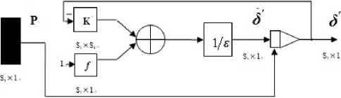
V. Analogue Circuit Experiment
0.5
-0.5
0.0
0.0
0.0
0.0 "
v1
Г-1.0'
-0.5
1.5
-0.25
-0.5
0.25
0.0
v2
0.0
0.0
-0.25
1.5
0.25
-0.5
0.0
и 3
Ы
0.0 г
0.0
-0.5
0.25
1.5
-0.25
0.0
v3
0.0
0.0
0.25
-0.5
-0.25
1.5
-0.5
u5
0.0
0.0
0.0
0.0
0.0
-0.5
0.5 _
u 6.
_ 0.0
First, this
paper
solves
this
question by using
improved Hopfield neural network based on the energy function of the neural network equals to the objective function of the finite element method and the minimum point, which is the stable equilibrium point of the network system, is the solution. In addition, the fig.10 gives the circuit. And then analysis is carried out for the accuracy and precision of computing method by comparing the results of calculation in the same initial condition separately.
IV. Conclusions
References Computing Method and Hardware Circuit Implementation of Neural Network on Finite Element Analysis
- N. G. Xie, T. T. Yu, W. D. Shao, “Network parallel algorithm in optimization computation of engineering structure," Journal of East China University of Metallargy, vol.18, no. 2, pp. 117-120, 2001 (in Chinese).
- W. L. Zhang. "Studying status and development of computing mechanics", Journal of Anhui institute of architecture, vol.9, no. 2, pp. 7-12, 2001 (in Chinese).
- X. Chen, D. H. Sun, H. Z .Huang, "Finite element system for structural analysis and neural network", Hoisting and conveying machinery, no. 6, pp. 6-8, 1999 (in Chinese).
- X. C. Wang ," Finite element method”, Beijing: Tsinghua University Press,2003 (in Chinese).
- D. H. Sun, Q. Hu, H. Xu ," Real-time Neurocomputing Model Used in Elastic Mechanics", China mechanical engineering,vol.8, no. 2, pp. 35-38, 1997 (in Chinese).
- H. B. Li, Neurocomputing based structural finite element analysis, Dalian: Dalian university of technology, 2003 (in Chinese).
- L. K. Cui, W. Wang, Z. Li, "Application of Hopfield neural network in finite element solving", Computer Engineering and Applications,vol.46, no. 16, pp. 46-47+49, 2010 (in Chinese).
- H. Z. Huang , H. B. Li, "Research on neurocomputing method on finite element analysis", Journal of Mechanical Strength,vol.25, no. 3, pp. 298-301, 2003 (in Chinese).
- E. Z. Liang, E. W. Liang, Circuit design and simulation application base on Protel 99 SE ,Beijing: Tsinghua University Press,2000 (in Chinese).
- Datasheet:“<0.4Ω CMOS 1.8V to 5.5V, SPST Switches ADG801/ADG802”. Analog Devices
