Constructing a model for managing the trajectories of innovative development based on their integral characteristics

Today, innovations are considered as the main driving forces of the modern economy in the sphere of production and services, and as the main factors of economic growth. Innovative way of development of the economy requires the use of appropriate methods to manage this development, both at the state and at the individual companies’ level. Innovations different in shapes and approaches to their implementation form are the basis for the development of business strategy, regardless of the legal form and size of the enterprise [1]. Therefore now the numerous enterprises face a question of developing a market-oriented business concept aimed toward a dynamic product policy and innovative development [2].

However modernization of traditional management methods by itself doesn't bring the expected efficiency. Development and search of the new concepts and approaches corresponding to essence of innovative processes is necessary.

In this regard, mathematical modeling that requires development of effective computing schemes, models and algorithms, is playing an important role [3–5].

We consider influence of the level of innovative development on a level of quality and economic efficiency of products.

We assume that the level of development of the trajectory of innovative product is equal to a product quality level, i.e. the coefficient of their relation is equal to 1.

Statement of the problem : it is known that in its activity any enterprise seeks to maximize the income and to minimize costs. Otherwise, the economic activities of a business are not practical.

Using a trajectory of innovative product development (TIPD), we define values of the income and costs functions and, as a result, we get an opportunity to calculate the optimum time of transition to other trajectory (criterion of transition - the greatest average economic efficiency for the studied time period).

The S-shaped curve describes development of the phenomenon during the growth stages, that is dynamic transition from one stable state when values of parameters of the phenomenon only became distinguishable and reached a minimum position (it is quite admissible that they could reach this position though a spike or a slow even increase), to other state, stable for some time, with the maximum values of parameters.

Processes which at first grow slowly, then accelerate, and then again slow down the growth, reaching to any limit, are rather widespread in economy. To simulate such processes the so-called S-shaped curves are used [6, 7].

Баркалов С.А., Аверина Т.А.

In Fig. 1, Fig. 2 the family of S-shaped curves and their derivatives are shown. Values of derivatives are always positive, i.e. functions of trajectories of innovative product development is monotonically increasing.

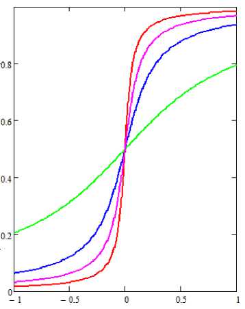
Fig. 1. The Family of S-curves

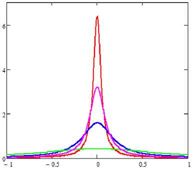
Fig. 2. Derived from S-shaped trajectories

Economic efficiency is defined as the ratio of profit to costs, and profit, in turn, is calculated as the difference of income and costs.

We assume that the value of the function of income at each time point is greater than the value of the cost function (i.e. the implementation of innovation can only result in positive economic effect).

Accordingly, based on the trajectory of product innovation development, we have to construct a function of income and costs. It is not possible to provide the necessary functions, by using only the function values of a trajectory of innovative development; therefore, we consider the integral characteristics of this curve [8, 9].

The algorithm of the model

We suppose there is some trajectory which is well known to the business entity. The trajectory will dominate in the industry during next period. The current status is known. However, the moment when the new product spreads in the industry is not determined. The difficulty is that the subject does not know when to begin investing in a TIPD x ₂ and how to deal with the possibilities of the TIPD x ₁ [3].

We construct functions of income, costs, profits and economic efficiency based on TIPD [8, 10]. We consider the trajectory of innovation development for the planning horizon T which is fixed and known. Values of the function X (t) at the initial time X (0) = Xо and the maximum level of development (technology limit) X(T) = Xmax are known X(0) = X0 [3]. In the future the process of trajectory development will be considered relative to the dimensionless axes. On the abscissa axis we measure the dimensionless time t = t/T, and we plot the dimensionless ordinates of the trajectory along the ordinate axis x (t) = X(t)/Xmax .

In Fig. 3 S-shaped developmental trajectory in dimensionless coordinates (the modified hyperbolic tangent function, x = 0.02, x = 1) is shown.

0 max

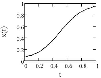
Fig. 3. S-shaped trajectory of development

Управление в социально-экономических системах

Plotting income, costs and profit functions is performed using the geometrical characteristics of plane figures. We consider figure bounded by a TIPD on time interval [0, 1] (Fig. 4). For this figure we introduce the following geometric characteristics: A – area; Sx , St – static moments concerning axes x, t respectively.

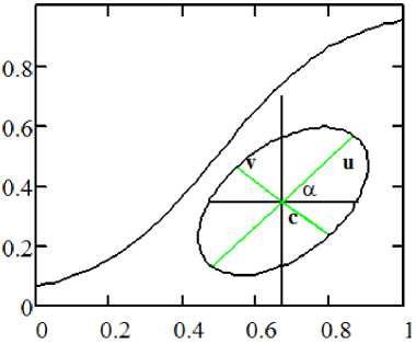
Fig. 4. Figure bounded by the trajectory of x ( t )

A = Ла dxdt , S x = Ла tdxdt , S t = Ла xdxdt .

The coordinates of the center of gravity of a flat figure is defined by the formulas:

tc

xc

S x A ,

S t A .

Principal axis passing through the figure center of gravity of the shapes shown in Fig.4.

The moments of inertia of a figure J , J and xc yc

the centrifugal moment of inertia J_txc of rather principal axes are defined through integrals:

J x= = Л A t 2 dxdt ,

J, = Ла x 2 dxdt ’

J txc = Ла txdxdt .

At turn of the principal axes on an angle α (against the course of an hour hand) the moments of inertia of rather new axes u, v are calculated on formulas [10]:

J., = J, sin2 a + JY cos2 a + 2 J^ sin a cos a, v      tc                 xctx

J„ = J, cos2 a + JY sin2 a-2 J^ sin a cos a,(4)

u      tc                xctx

J = (J, - JY )sin a cos a + J^ (cos2 a-sin2 a). uv       tc      xctx

The formulas (4) show that while the angle a value of the moments of inertia changes, the sum of the axial moments of inertia concerning such coordinate axes remains to a constant.

^Jt = ^{+ J}x = = ^Ju ^{+ J}v .

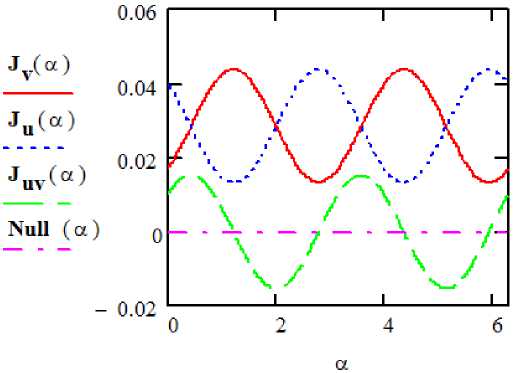
Fig. 5. Fluctuating of the moments of inertia when turning axis at an angle α

Therefore, if concerning one axis value of the moment of inertia is maximum, then concerning other axis, perpendicular to it it’s the minimum. Besides such axes the centrifugal moment of inertia J_uv is zero. In Fig. 5 dependences (4) are presented in the graphic form (the angle a changes from 0 to 2 n ). From the schedules of Fig. 5 it is visible: in the points where J_v – is maximum, J_u – is minimum, and J = 0 . uv

The central axes concerning which the centrifugal moment of inertia is equal to zero, and the moments of inertia reach the maximum and minimum values, are called the principal central axes of inertia [10].

Баркалов С.А., Аверина Т.А.

We show that the problem of determining the positions of the principal central axes of inertia and calculation of the principal moments of inertia is a problem on eigenvalues.

We designate through M a matrix of the moments of inertia, and through V a vector of the directing axis cosines v :

M =

J t_c

Jtxc l = cos a , m = sin a, l2 + m2 = 1.

Then the first of formulas (4) can be written down in the form:

J = V T MV ^v V^TV ^.

The expression (7) is called Rayleigh's quotient [11].

We consider the eigenvalue problem

MV = 1 V .

According to Rayleigh's principle, the relation (7) is minimized by the first eigenvector V1 , and this minimum value is equal to the smallest eigenvalue 11 of a task (8). The maximum of the relation (7) is reached on eigenvector V2, and this maximum value is greater eigenvalue 12 [11].

Own vectors – the directing cosines of the principal axes of inertia.

V =

l ₁

.^m 2 J

, V 2 =

l ₂ m ₂

In these axes the matrix has a diagonal form, i.e. relatively to the principal axes of inertia the centrifugal moment of inertia is zero.

The principal moments of inertia are determined by the condition of equality to zero matrix determinant:

	Jt -1    Jtx tc                 txc	1
det		= 0
[	Jtxc    Jxcc - 1	J

And are calculated according to the formulas:

J min =1 1 = 2 J x c + 2 J t c - 2V ^JX c ² — 2 ^Jx J + ^Jt c ² + 4 J ²,

1   112        22

Jmnx =1? = —Jy +--Jf +--J^x  — 2 Jy Jt + Jf  + 4 Jtx.

max 2    2  xc    2  tc    2     xc         xc  tc     tctx

It is easy to see that the sum of the principal moments of inertia is a constant ^J max ^{+ J} min = ^Jx_c ^{+ J}t_c ^.

The directing cosines of the principal central axes of inertia are defined as:

s 1 =

J tx_c

, ₁

t_c     min

s ₁

7^{1+ s} 12

7¹+ S 1 ²

s 2 =

J tx_c

J -J t_c     max

s ₂

7^{1 +} s 22

1 + S 22

As eigenvectors of a symmetric matrix are orthogonal, the principal axes of inertia are mutually perpendicular.

We consider such characteristic of a flat figure as the principal radiuses of inertia.

Управление в социально-экономических системах

On the principal central axes of inertia we construct an ellipse, the maximum and minimum radiuses of which are determined by formulas:

i max

i min

These values along with coordinates of the center of gravity of a figure are used to construct functions of the income and costs according to TIPD.

In Fig. 6 the principal central ellipses of inertia of corresponding curvilinear trapezoids for various intervals of time are shown.

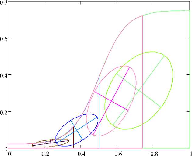
Fig. 6. Principal central ellipses of inertia

All above-mentioned geometrical characteristics are the integrals of the form (15).

I_pq = IL t^Px^qdxdt .                                                                         (15)

Calculation of integral on the area is reduced to calculation of integral on a contour and the trajectory is approximated by the set of linear functions. A conclusion of universal formulas for calculation of geometrical characteristics of flat figures on the basis of Green's formula is presented in [10]. The algorithm is realized in the Mathcad system.

Algorithm of construction the functions of the income and costs:

• 1.    Divide the time axis by a discrete set of points.

• 2.    Select the figure bounded by trajectory.

• 3.    We receive the corresponding points on curves.

• 4.    Further we fix t 2 time point.

• 5.    Repeat the steps for the subsequent time spans.

In an initial time point all characteristics are known.

We consider a trajectory on the interval [ t 0 , t 1 ].

We calculate geometrical characteristics and the corresponding values of functions of the income and costs for a curvilinear trapezoid.

We consider a curvilinear trapezoid on the interval [ t 0 , t 2 ].

We calculate geometrical characteristics and values of functions for the appropriate shape again.

Graphic interpretation of the algorithm is presented in Fig. 6. There are principal central axes of inertia and corresponding central ellipses of inertia with radiuses for each curvilinear trapezoid.

Баркалов С.А., Аверина Т.А.

We introduce the following hypothesis: the income (I) of the implementation of innovation depending on TIPD x ( t ) in time t is defined by the formula (16) and costs (C) – by the formula (17). Then the profit (P) from the implementation of innovations in time t is defined by the formula (18) and economic efficiency (EF) – by the formula (19):

Income I = - max , x_с ²

Costs c = - min- , t с 2

Profit P = I — C = - max- — i min , x с 2      t c 2

P

Economic efficiency EF = —:

Г 2    2. )

max    i min

—

X ²    2

V x c      t c )

² min t с ²

.

Graphs of functions income, costs, and profit for a discrete set of nested time intervals are presented in Fig. 7. The function of the economic efficiency is shown on the second ordinate axis.

The trajectory (Fig. 8) is set by the function (20):

x ( t ) = x 0 +( xk

—

x o )

[ t^+11

V 2    2;

P = k - x o - u - ^— q - ,

• k_i – is a constant;

• u_i – value of resources along the trajectory;

• x_k – value of the trajectory in a finite time;

• x ₀ – value of the trajectory at the initial moment of time;

• P _- - speed of the trajectory development;

q_i – loses during the transition to the subsequent trajectory.

We assume the following parameters of the TIPD:

k_x = 50; u 1 = 3; X k 1 = 1;

• x o 1 = 0.02; ₽ i = 3; q i = 0.

  

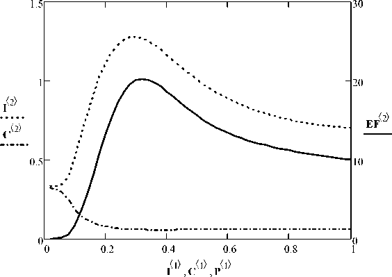
  Fig. 7. Average income (I), costs (C) and economic efficiency (EF)

  
  
  

  t

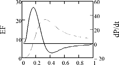
  Fig. 9. Economic efficiency (EF) and speed of its change

  
  
  
  
  

t

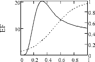
Fig. 8. The trajectory x ( t ) and economic efficiency (EF)

Управление в социально-экономических системах

In Fig. 9 is a graph showing changes of the economic efficiency and the rate with which the effectiveness changes (a derivative of efficiency in time (right axis)).

Maximum economic efficiency is achieved at t = 0.32 and equals to 20.277. The average economic efficiency over the study period is 11,471.

Conclusion

On the basis of the offered model it is possible to analyze functions of the income, costs, economic efficiency, to define the optimum time moment of starting new trajectories, in this case the requirement of continuity and convexity is not required.