Construction of approximate mathematical models on results of numerical experiments

The present mathematical modeling level allows us to construct the models of very complex processes and to make a detailed numerical experiment. As a rule, the numerical implementation of such mathematical models involves time-consuming. In some cases, calculation results of processes characteristics are required in real time. This can be the movement control of any objects or any process. Having information on the results of numerical or natural experiment we can construct mathematical models with lower dimension, which reproduce the characteristics of these processes by small time consuming. We consider the example of mathematical models dimension reduction. This example is related with numerical modeling of artillery shot, which is characterized by the diversity of occurring physical, chemical and gas-dynamic phenomena. In various barrel systems tests the operative analysis of a natural experiment is very important in order to improve the accuracy characteristics and identification of using calculation methods.

• 1.    Mathematical Model of the Shot

The movement of burning gunpowder elements along the barrel at the shot is a classic case of heterogeneous system movement, due to processes of heat and mass exchange and friction between the phases [1].

The main assumptions of the model:

• 1)    distances, at which the flow parameters vary considerably, much more than distances between the particles and size of the particles;

• 2)    various phases are present simultaneously at all points of space, at the same time each phase occupies a portion of the mixture;

• 3)    calculation of each phase movement can be performed independently from the mixture under the condition that appropriated account of the interaction between the different phases is provided;

• 4)    viscosity and thermal conductivity is significant only in the phases of interaction processes;

• 5)    particles have the same size on average, collisions, or interaction between the particles, can be neglected;

• 6)    phases movement is one-dimensional;

• 7)    heat transfer to the burning surface of the grains is not taken into account (heat wave movement velocity in the gunpowder equals to burning velocity);

• 8)    material of the particles is incompressible;

• 9)    gas parameters inside and outside of the gunpowder elements are same in this cross-section.

The system of one-dimensional hydro-mechanical equations describing the barrel system ballistics in terms of mechanics of heterogeneous medium has the form [1]:

∂ρmS ∂ρmSv

∂t ∂x

= SG,

д6 (1 — m) S d6 (1 — m) Sw m Iй = —SG, ∂t∂x

• "7 । dpmSv2 = -mSdp । SGw - STw - ncTic, ∂t ∂x∂x

• d$(1-m)Sw + 86 (1 - m Sw = — (1 — m Sdp — SGw +   -(i)

∂t             ∂x∂x

dpmSe dpmSev d [mSv + w (1 — m) Sw]           (v — w)2

— + ^dx- = p^---dx——+ SG Q + ^-

I

+Stw (v — w) HcTicV — Hcqc,

∂ψ ∂ψ S 0

di + wax = Л" w u

p(1 — ap) = (k — 1) p£, where t is time; x is coordinate; ρ is gas density; m is mixture porosity (volume of voids per unit volume); S is variable cross-sectional area of the chamber and the barrel; v,w are movement velocities for gas and solid phase in the barrel respectively; G is gas coming per unit volume; δ is density of gunpowder material; p is pressure; τw is hydraulic resistance of gunpowder elements per unit volume; Пс is perimeter of the barrel; t1c,t2c are friction force of gas and gunpowder particles on the barrel surface per unit area respectively; ε is internal energy per unit mass of gunpowder gases; Q is heating value (potential) of gunpowder; α is covolume; qc is heat flow to the barrel surface; ψ is the relative proportion of burnt gunpowder; Л0, S0 are the initial volume and surface of grain gunpowder; a (^) is current burning surface to original ratio; u is the linear velocity of gunpowder burning; k = Cp is adiabatic index; cp,cv are heat capacity of gas at constant volume and pressure respectively.

Received system of equations contains seven variables: gas parameters p, ρ, ε, v , solid phase velocity w , the mixture porosity m and relative share of burnt gunpowder ψ .

Initial and boundary conditions:

0 < X <  L km ,

t = 0,

v = w = 0, p = Pn, E = En =

f θ^,

^ = ^n;

x = 0,   t > 0,   v = 0;

x = Xcn,   t > 0,   v = Vcn.

Boundary movement x = xcn and projectile velocity are determined by the equations of projectile movement:

dv _cn ^q dt

= S cn ⁽P - P pr ) - F t 1

dx _cn dt

⁼ v cn ^,

where L _km is length of the chamber; f = RT v is gunpowder force; R is gas constant; T v is the gunpowder burning temperature at the constant volume; 9 = k — 1 ; q is projectile mass; F _t is resistance force during the projectile movement in the barrel; S _cn is area of the barrel; p _pr is compressed air pressure in front of the projectile (back pressure); v _cn is projectile velocity; x cn is the path of the projectile in the barrel; p n , ε n , ψ n are the initial values of the relevant parameters.

Since the share of friction and heat transfer to the surface of the barrel in the total balance of momentum and energy of the shot is small, we can use the approximate dependencies neglecting the contact heat transfer and friction of particles on the barrel:

qc = Nuy (T — Tc), Tc = Tic = 0.125(pv |v|, T2c = 0, dk where Nu is Nusselt number; λ is thermal conductivity coefficient of gunpowder gases; T is temperature of the gunpowder gases; Tc is surface temperature of the barrel, dk is barrel diameter; ξ is resistance coefficient of the gunpowder grains in the layer.

Surface temperature of the barrel is defined by the equation:

dn 2    /NuA\² _  _    ^.2

dt = Слад( - n-vn) ,n( )= ’ where n = (Tc - Tn), Tn is initial temperature of the barrel surface; cc,5c,Xc are heat capacity, density and thermal conductivity of barrel material.

The air initially located in the chamber and the heating particles entering the flow with the gaseous igniter burning products and creating considerable heat flows deposited on the gunpowder surface are taken into account to describe the ignition process. In the gas-dynamic system of equation, which takes into account the gradual ignition, it is additionally accepted:

• 1)    burning products of various parts of the charge, igniter and air are the homogeneous non-reactive mixture with the same velocities, pressures and temperatures;

• 2)    the gases nature for different brands of igniter is the same;

• 3)    grains of the igniter move with gunpowder elements;

• 4)    inner and outer surfaces of the gunpowder elements in a given section are ignited at the same time;

• 5)    deposition of incandescent particles in ignited part of the charge is neglected;

• 6)    gunpowder burning velocity is determined on the basis of approximate methods of non-stationary and erosive burning [1].

• 2. Numerical Solution of the Model Equations

Conjunction Euler–Lagrange (CEL) method [1] is used for the numerical solution of equations (1). The scheme of this method belongs to the class of homogeneous conservative schemes that by introducing pseudoviscosity allow to keep "through" account of gasdynamic parameters in the shock waves presence. Pseudoviscosity component included in the pressure and "smears" the shock wave front on several intervals of grid, so that the values of the functions vary continuously passing through the leap and satisfy conservation law of Rankine–Gyugonio. The upstream differences are used to approximate the convective terms. Due to shifted grids, CEL-method has the second order of accuracy, which ensures fast convergence of the solution regarding to the step along the coordinate.

To simplify the model (1), (2) we consider the processes occurring in the shot, by assumption that pressure, density and temperature of gas are taken average over the burning chamber volume. Accounting of combustion products movement will be made on the bases of some functions selected on the results of numerical simulation for solutions of equations (1), (2). For average over volume parameters we have the following system of ordinary differential equations [2]:

Wdp = dt

-----M (xTp - T) + 1 — ap

kp

P (1 — ep)

[ M (1 — 0)

-

S cn v cn ρ c

,

Wp dT

T dt

M (XTp — T) ' \ [M f1 — t) — Scnvcnpc] , p (1 — ep) L   X о /             J

de dt = u,

dW       M

dt    Scnvcn + о ,

back of projectile space p c = ---- a +

as well as equation (2).

Here W is free volume of the chamber and the barrel; T _p is isobaric temperature; χ is heat loss coefficient; ρ c is density behind the projectile associated with pressure p c in

RT ; M = 8uL is gas coming from combustion products; p c

X (e) is relationship between the burning surface area and thickness of the burnt body;

gunpowder burning velocity is determined by the dependence u = u 1 p ; u 1 is unit burning velocity.

We introduce the vector of correction functions Ф = [^ (e) , ^ _x (t) ,^ _c (t), ^ _u (e)] T , responsible for the approximation of the model (3) to the mathematical model (1):

S = ^sSo -;

pϕ c

pc =

-

x = x o ^ x ;

^{w0 (1} - ^f 1 ^{(x)) v} 2 n

2W k x

1 + £л (x) 2q

;

u = u i ^ u p;

02 - 1

f (x) = 0.

Here 0 = Sk-; Wk = SkLk is combustion chamber volume; Sk ,Lk are sectional area Scn and length of the combustion chamber; x = cn^—-Lk

.

The controls ϕ Σ , ϕ u have meaning for e ≤ e k and therefore are accepted depending on the size of the burnt body. The value of £ 0 = — in (4) is determined by the mass of e k charge ω and body thickness e k .

During burning it is assumed that igniter has the same burning velocity as gunpowder, and the area of the burning surface depends on the thickness of the burnt body v             - 2eV wU  6w D.\   Dw) ’ where ww ,5w, Dw are mass, density, diameter of igniter particulars. The typical value x0 = 0,9. Initial values for equations (3), (8): p (0) = pn,T (0) = Tn,e (0) = 0, W (0) = Wn, vcn (0) = 0.

Dependencies P (t) = p (t), P c (t) = p c (t), V cn (t) = v _cn (t) obtained by numerical solution of equations (1), (2) are used to calculate the functions Φ . Functions Φ should ensure the minimum values of the deviations of variables p (t), p c (t), v cn (t) , calculated for equations (3), (8) from values P (t), P c (t), V cn (t) for the time of the shot t - :

t _k

J p ( Ф ) = /

[p (t) — P (t)]2 dt ^ min, Φ tk

J Ф /

[pc (t)

— P _c (t)] ² dt ^ min, Φ

J v

t _k

( ♦ ) = /

[v cn (t) — V cn (t)] ² dt ^ min .

Φ

After substituting expressions (4) – (7) in equations (3), (8) we obtain a system of ordinary differential equations for the phase variables X = (p, T, e, W, vcn)T with the control Φ. The system of equations (3), (8) together and conditions for minimum of functionals (9) represent the optimal control problem. The system of equations (3), (8) is solved numerically by the Runge-Kutta method with fourth-order accuracy with a step At. Controls Ф are replaced by linear functions on intervals of time and the burnt body [tj, tj+1] , t0     0, tNф     tk; [ej, ej+1] , e0    0, eNф     ek•

Φ - Φ

ф (y) = Ф +---------"(y - yj), j = 0,N - 1, y =(t,e), yj+1 - yj where NΦ is number of intervals. Thus the optimal control problem is reduced to the finitedimensional problem of multicriteria optimization to determine the values Φj . Multicriteria optimization problem is solved by use of a hybrid multipopulation genetic algorithm [3].

We consider the following algorithm, which does not require the introduction of additional sub-populations and user interaction in the choice of optimal Pareto solutions [3].

Suppose we are given the problem of multi-criteria optimization:

F (x) ^ min, or

Fi (x) ^ min, i = 1, N.

Just as in the case of one criterion the population by given size R is formed. From this population the individuals (solutions x ) are chosen, that are the bests for each of N criteria with criteria values

Fi (x) ,i = 1Л.

Individual, a leader in a given population, is defined by the rule:

x0 = arg min I max | Fi (x) j=1,R i=1,N

-

F (x)|)] .

Selecting for crossing is carried out by the tournament. Solution obtained in a result of a number of iterations is unique and Pareto optimal. Genetic algorithm with a real encoding is used as an optimization method.

Fig. 1 shows relationships P (t), P c (t) , obtained from the numerical solution of equations (1), (2) and used as a standard for the selection of corrective functions Φ (black circles show pressure on the bottom of the channel, light circles show pressure on the bottom of the projectile). Fig. 2 shows dependence V cn (t) (black circles). Relations p (t) , P c (t), v cn (t) , calculated on equations (3), (8) according to corrective functions, are shown at the same figures (bold line in fig. 1 shows pressure on the bottom of the channel, light line shows pressure on the bottom of the projectile). Velocity of the projectile v cn (t) in fig. 2 is a bold line.

As you can see, the selection of the corrective functions provides reproduction of firing process in the basic details. Change of correction functions is shown in fig. 3: ϕ Σ _e ^e _k is dependence 1; ϕ χ _t^t _k is dependence 2; ϕ c _t ^t _k is dependence 3; ϕ u _e ^e _k is dependence 4.

Let us consider the following level of dimension reduction of mathematical model – approximation of point features. On the example of artillery shot it is the dependence of the maximum pressure pmax in the chamber and muzzle velocity vcmnax from the initial process parameters (vector z = (pmax, vCnax)T). As the impact parameters we consider

Fig. 1. Pressure curves at the bottom of the channel and the bottom of the projectile

vector Y = (T p , e k , u 1 ,5, x 0 ) in the range [0.95; 1.05] of nominal values. Under the random distribution of the parameters Y from the solution of equations (3), (8) for given values

Fig. 3. Correction functions

of the correction functions Ф we obtained H = 1000 points ( z , Y ) j , j = 1,H . On these data we carry out comparative analysis of different approximators:

• 1)    multiple regression equation;

• 2)    support vector method;

• 3)    multilayer neural network;

• 4)    radial network;

• 5)    the method of fuzzy decision trees.

Multiple regression equation is z = b + ( w , Y ) , where the coefficients b, w are found by the method of least squares.

In support vector method z ( Y ) = ^ H=1 (A h — A h ) K ( Y , Y ^h ) + b , summation is carried out for (A h — A h ) = 0 , where K ( Y , Y ‘ ) = exp ( -0, 5( Y — Y ‘ ) T a ^-1 ( Y — Y ‘ ) ) is a kernel function. Coefficients λ ^∗ _h , λ _h , which are Lagrange multipliers in the quadratic programming problem, are calculated iteratively [4] on available data set, σ is a covariance matrix.

In multilayer neural network the input signal is converted by the layers according to the expressions:

u _i ^k

N k - 1

= ^ wjqk-1 ’ qk = g(uk)’ i =1,Nk’ k = 1,KC’ g(u) = j=0

1 + exp(—ви) ’

• q ⁰ = Y , z = q ^Kc ,

  where N k

  
  

is the number of neurons in the kth layer; Kc is the number of layers in the neural network; wkj are weighting coefficients; g (u) is activation function with optimization parameter β .

Radial network performs conversion z ( Y ) = ^ L ₌₁ w _h exp — " Y_{2< y} C h " ] , where L is the number of centers of radial neurons with values C h ; coefficients w h , σ h are determined by training.

In the method of fuzzy decision trees the decision tree [3] is constructed on a data set. Constructed decision tree is considered as a set of fuzzy rules by the form

R r ^:    if f") Y j £ A jr then z is B r , r = 1, K R .

Condition Y j ∈ A j _r corresponds to the separation of the set of points on the breakdown Y j ^≥ _< w j and means entering of value Y j in the fuzzy intervals on the left and right of parameter w j with the give n m embership functions. For a given vector Y the degrees of truth for each rule a r , r = 1,K r , are defined. As a result, an aggregated output signal is determined by formula:

z ( Y ) =

K r =1 α r

K R            n

52 ar Wro + 52 Wrj Yj • r=1             j=1

Selection of 1000 points is divided into the training selection (750 points) and the test selection (250 points). On the test selection the standard error was calculated for each approximator. The results are given in table. The best result was shown by the radial

Table

The standard error

Approximator pmax max vcn 1 10,43 5,07 2 3,23 4,32 3 3,88 4,45 4 2,28 4,05 5 6,89 5,05 network. Error for maximum pressure pmax is 2,28 MPa or 0,52%, for muzzle velocity vcmnax error is 4,05 m/s or 0,43%. Number of centers of radial functions is L = 100, ah = 2. The linear dependence (1st approximator) showed the worst results. This is well illustrated by the graphs for comparing of the approximated value pamax with pmax calculated from equations (3), (8). Fig. 4 corresponds to the linear approximator, and fig. 5 corresponds to the radial approximator.

Conclusion

Application of the methods of knowledge and data extraction, and genetic algorithms allows us to construct the adequate mathematical models that can be implemented in various control systems.

Acknowledgements. The research was done under the state assignment No 1.1481.2014/E, registration number is 114072170012 from 21.07.2014.

Fig. 4. Comparison of the approximated and calculated pressures (linear approximator)

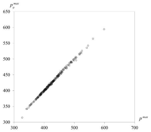
Fig. 5. Comparison of the approximated and calculated pressures (radial approximator)