Construction of high-precision low-dimensional MgFE using local approximations and generating FE

In modern aviation and space rocket technology, elastic structures, plates, beams, and shells with a non-uniform (fibrous) structure are widely used. When analyzing the strain-stress state (SSS) of elastic structures (bodies), the finite element method (FEM) is actively used [1–7]. Basic discrete models (BM) of bodies, which take into account their inhomogeneous and micro-inhomogeneous structure within the framework of the micro-approach [8] using finite elements (FE) of the first order, have a very high dimensionality.

In order to reduce the dimensions of discrete models, the method of multigrid finite elements (MMFE) [9–11] is very effectively used. MMFE is used especially effectively in solving problems of the theory of elasticity [12–16] for composite bodies (CBs). The MMFE is implemented based on the Lagrange functional (i.e., in displacements) [17] using multigrid finite elements (MgFE) [18–21]. Since when constructing an n - grid FE, not one but n nested grids (n > 2 ) are used, the MMFE can be considered as the generalization of the FEM, i.e., the FEM is a special case of the MMFE. It follows herefrom that if in the calculations of bodies by the FEM, MgFEs are used; the MMFE is practically implemented in this case. Inhomogeneous, microinhomogeneous structures of CBs are taken into account within the framework of the microapproach using the MFE. The existing approaches and numerical methods for solving elasticity problems for CBs have complex formulations and are difficult to implement [22–30]. For bodies with an inhomogeneous regular structure with different filling factors, which, from the point of view of the macro approach, are considered as isotropic homogeneous bodies, the SSS is determined using fictitious elastic moduli. The procedures for finding fictitious elas- tic moduli are shown in [31] for two-dimensional composites, and in [32] for three-dimensional ones. The main advantages of MMFE are that it generates low-dimensional discrete models for CBs and is implemented on the basis of FEM procedures.

When constructing a multigrid finite element (in short, a standard MgFE) using known procedures, a fine grid and large grids nested in a fine one are used. The small (basic) grid is generated by the basic partition, which takes into account the heterogeneous, micro-homogeneous structure of the standard MgFE, large grids are used to reduce its dimension. For standard MgFEs the following is typical. Any large grid of a standard MgFE and corresponding approximations of displacements are determined on its entire region. This leads to an increase in the dimension of the standard MgFE with an increase in its order of accuracy, since in this case high-order displacement approximations are used on large grids. To reduce the error of approximate solutions, (standard) high-order MgFEs (MgFEs of high order of accuracy) are used, which have a high dimension. Nevertheless, the use of high-precision MgFE s is difficult, since they generate discrete models of high-dimensional bodies.

The main disadvantage of the FEM and MMFE is that when constructing solutions with a small error for a CB using the well-known single-grid FE, MMFE, discrete models of high-dimensional bodies must be used when constructing solutions using the FEM, MMFE with a small error. To solve this problem, it is proposed to use high-precision small-scale MgFEs, which make it possible to determine stresses with a small error for large discrete CB models.

In this paper, we propose a method of local approximations (MLA) for constructing high-precision low-dimensional MgFEs (briefly, small-dimensional MgFEs), which are used in the calculation of the SSS from the MMFE of elastic homogeneous and CB. The MLA is used for the CBs that satisfy the following basic provisions.

Postulate 1. The CBs consist of heterogeneous isotropic homogeneous bodies, the connections between which are ideal, i.e., on the common boundaries of heterogeneous isotropic homogeneous bodies, the functions of displacements and stresses are continuous.

Postulate 2. Displacements, deformations and stresses of multimodular isotropic homogeneous bodies correspond to the Cauchy relations and Hooke's law of the three-dimensional problem of the linear theory of elasticity [16].

It should be noted that MLA, in fact, generates new approaches to the construction of the MgFE. Two approaches are considered, i.e., two types of small-sized MgFEs. Small-sized MgFEs of the first type are designed on the basis of standard ones using local approximations of displacements, which are determined on subdomains of standard MgFEs. Small-sized MgFEs of the second type are designed using generating FEs. The brief essence of the construction of small-sized MgFEs of the first type is as follows.

According to the MLA, in the central part of the V ₀ domain of a standard MgFE, high-order local approximations of displacements (built on large grids) are used, in the vicinity of the V ₀ region boundary, low-order approximations are used, which makes it possible to design a high-precision MgFE V_p of small dimension, i.e., a small-sized MgFE of the first type, the dimension of which is equal to the dimension of the standard one. The following should be noted. With an increase in the order of accuracy of the MgFE V_p , its dimension does not change, i.e., it does not increase, and therefore it is called a high-precision MgFE of small dimension. The procedure for constructing small-sized MgFEs of the first type is described in detail. As is commonly known, the calculation of the static strength of elastic structures is reduced to finding the maximum equivalent stresses for them, the determination of which with a small error for CB is currently an urgent problem.

The calculations show that small-sized MgFEs of the first type generate maximum equivalent stresses in a CB, the errors of which are 25–50 times less than the errors of similar stresses obtained using standard MgFEs, which have the same shapes, characteristic dimensions, dimensions, inhomogeneous structure and form the same discrete models as low-dimensional MgFEs. The given example of the calculation of a CB by MMFE with the use of small-sized MgFEs of the first type shows their high efficiency.

The main advantages of small-sized MgFEs of the first type are as follows. Firstly, small-sized MgFEs of the first type generate maximum equivalent stresses in CBs with a smaller error than standard ones, and form discrete models of small-scale CBs. Secondly, the use of small-sized MgFEs of the first type in the calculations by MMFE allows determining the maximum equivalent stresses with a small error for large discrete CB models. It follows from this that small-sized MgFEs of the first type are more efficient than standard ones (on the basis of which small-sized ones are built).

The procedure for constructing small-sized MgFEs of the second type based on standard high-precision MgFEs with the use of generators of the FE is briefly shown. The small-sized MgFEs of the second type have the same order of accuracy as the standard ones, but their dimension is less than that of the standard ones. Therefore, small-sized MgFEs of the second type generate discrete CB models of a smaller dimension than standard ones.

1. Procedure for constructing standard multigrid finite elements

Without losing the generality of judgments, we will show the main provisions for constructing standard MgFEs based on the Lagrange functional using the example of a Lagrangian two-grid finite element (2gFE) with the dimensions 8 h x 8 h x 8 h (Fig. 1), h is given.

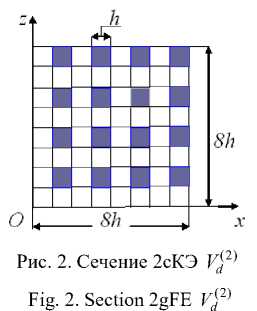
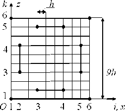
Here and below, the MgFE in the figures are shown in the local Cartesian Oxyz coordinate system. The considered 2gFE Vd²^ is reinforced with continuous fibers with a cross section h x h that are parallel to the Oy axis and the distance between them is equal to h . Fig. 2 shows the 2gFE section in the Oxz plane, the fiber sections are shaded. We believe that between the components of the inhomogeneous structure 2gFE bonds are ideal, and the functions of displacements, stresses, and strains of these components satisfy Hooke's law and Cauchy's relations, corresponding to the three-dimensional problem of the linear theory of elasticity [12–16]. That means that three-dimensional SSS is realized in the entire 2gFE V_d ⁽²⁾ region [16]. The 2gFE V_d ⁽²⁾ region is represented by a BM R_d consisting of homogeneous single-grid FEs (1gFEs) V_j^h of the first order in the form of a cube with the h side [6; 7], j = 1,..., M ; M is the total number of IgFEs V j , for fig. 1 we have M = 512. Fig. 1 shows BM R d 2gFE V d^ , which takes into account the inhomogeneous structure of 2gFE V d²² and generates a fine (basic) nodal uniform grid h_d of the dimension 9 x 9 x 9 with the step h .

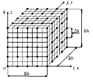
Рис. 1. Сетки 2сКЭ V_d ⁽²⁾

Fig. 1. Grids 2gFE V_d ⁽²⁾

On the hd fine grid, we determine the Hd2 large uniform grid with the 5 x 5 x 5 dimensions with the 2h step. In figure 1

Hd(2) large the grid nodes are marked with dots – 125 nodes. The Пd total potential energy of the basic partition Rd 2gFE Vd(2) (i.e., the Lagrange functional [17]) can be represented in matrix form [6; 7]:

M

П d = ∑ (¹ q ^T j [ K^h j ] q j - q ^T j P j ) ,                                   (1)

j = 1 2

where [ K^h_j ] – rigidity matrix; P _j , q _j – vectors of nodal forces and unknown 1gFE V_j^h ;

T – transporting; М – total number of 1gFE V_j^h .

With the help of Lagrange polynomials [6] on the H_d ⁽²⁾ grid, we determine the u ₂, v ₂, w ₂ approximating functions u ₂, v ₂, w ₂ for the displacements u , v , w of 2gFE V_d ⁽²⁾ , which we write in the form

555       555        555

u 2 = ∑∑∑ N ijk u ijk , v 2 = ∑∑∑ N ijk v ijk , w 2 = ∑∑∑ N ijk w ijk ,          (2)

i = 1 j = 1 k = 1                           i = 1 j = 1 k = 1                            i = 1 j = 1 k = 1

where u_ijk , v_ijk , w_ijk – desired values of the functions u ₂, v ₂, w ₂ in the node i , j , k of the H_d ⁽²⁾ grid; i , j , k – coordinates of the desired function values ijk , which is introduced for H_d ⁽²⁾ large grid nodes (Fig. 1); N_ijk = N_ijk ( x , y , z ) – basis function of the node i , j , k of the H_d ⁽²⁾ grid, i , j , k = 1,...,5 where

N ijk = L i ( x ) L j ( y ) L k ( z ),                                         (3)

∏ ⁵ x - x ⁵ y - y ⁵ z - z

α ; Lj(y)= ∏ α ; Lk(z) = ∏ α , xi,yj,zk – coordinates α=1,α≠i xi - xα            α=1,α≠ j yj - yα            α=1,α≠k zk - zα of the node i, j, k of the Hd(2) grid in the Oxyz coordinate system.

Let us denote: N _β = N_ijk , u _β = u_ijk , v _β = v_ijk , w _β = w_ijk , where i , j , k = 1,...,5, i.e., β = 1,...,125.

Then expressions (2) take the following form

125                 125125

u2=∑Nβuβ, v2=∑Nβvβ, w2=∑Nβwβ.(4)

β=1                β=1

Let us denote: qd = {u1,...,u125, v1,...,v125, w1,..., w125}T – nodal displacement vector of the Hd(2) large grid, i. e., the vector of unknown 2gFEVd(2) . Using (4), the qj vector components of the nodal unknowns 1gFEs Vjh we express in terms of qd vector components. As a result we obtain qj=[Adj] qd,(5)

where [ A^d_j ] – rectangular matrix; j = 1,..., M .

Substituting (5) into expression (1), from the condition ∂ П_d / ∂ q _d = 0 we obtain a matrix relation of the form[ K_d ] q _d = F _d , where

MM

[ K d ] = ∑ [ A^d j ] ^T [ K^h j ][ A^d j ], F d = ∑ [ A^d j ] ^T P j ,                          (6)

j = 1                                     j = 1

where [ K_d ], F _d – rigidity matrix (dimensions - 375 × 375 ) and nodal force vector (dimensions – 375) of the standard 2gFE V_d ⁽²⁾ .

The peculiarity of standard MgFE lies in the fact that any large grid of a standard MgFE and the displacement approximations corresponding to it are determined over its entire domain.

A standard 2gFE of the cube shape, which has a uniform large grid of the dimensions ( n + 1) x ( n + 1) x ( n + 1), is called a 2gFE of the n‘ h order. Since the uniform large grid H ² of 2gFE V^ has the dimensions 5 x 5 x 5 , 2gFE V (²^ is called 2gFE of the fourth order. Note that the dimensions of the Lagrangian 2gFE of the n^th order of the cube shape when using a large uniform grid are3( n + 1) ³ , i.e., with the increase in the order of n , the dimension of the 2gFE sharply increases.

Comment 1. The solution constructed for the H_d ⁽²⁾ large grid of the 2gFE V_d ⁽²⁾ is projected onto the fine h_d grid of the basic partition R_d of 2gFE using the formula (5), which makes it possible to calculate the stresses in any 1gFEs of the R_d partition , therefore, it is possible to determine stresses in any component of the inhomogeneous structure 2gFE V_d ⁽²⁾ .

Comment 2. By virtue of (5), the dimensions of the q _d vector (the dimensions of 2gFE V_d ⁽²⁾ ) do not depend on the number М , i.e., on the dimensions of the R_d partition. Therefore, to take into account a complex inhomogeneous (microheterogeneous) structure in 2gFE V_d ⁽²⁾ , arbitrarily small basic partitions R_d consisting of 1gFE V_j^h can be used. In this case, the 1gFE V_j^h describes the threedimensional stress state as accurately as desired (without simplifying hypotheses).

Comment 3. We note the case when a 2gFE V_d ⁽²⁾ has a complex shape and its large grid has external nodes that coincide with the nodes of large grids of neighboring 2gFE V_d ⁽²⁾ . In this case, when constructing a 2gFE V_d ⁽²⁾ at all nodes of its fine grid, the desired displacements u , v , w are expressed in terms of nodal displacements of the H_d ⁽²⁾ large grid of 2gFE V_d ⁽²⁾ , except for those nodes of the fine grid that coincide with the nodes (with docking nodes) of the large grids of neighboring 2gFEs and the H_d ⁽²⁾ grid, which ensures the docking of 2gFE V_d ⁽²⁾ with the neighboring 2gFEs.

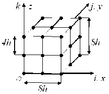
Рис. 3. Крупная сетка H_d ⁽³⁾

Fig. 3. Large grid H_d ⁽³⁾

When constructing a (three-grid) 3gFE, we use a finite number of 2gFEs, their large grids form a fine 3gFE grid, on which we determine a large grid for 3gFEs. The procedure for constructing a 3gFE is described in [9; 19]. Let us consider a special case when the construction of the 3gFE V_d ⁽³⁾ is carried out on the basis of one 2gFE V_d ⁽²⁾ . We consider the H_d ⁽²⁾ large grid of 2gFE V_d ⁽²⁾ to be the fine grid 3gFE. On the H_d ⁽²⁾ grid for the 3gFE V_d ⁽³⁾ we define the H_d ⁽³⁾ large grid. In figure 3 nodes of the H_d ⁽³⁾ uniform grid with the step 4 h are marked with dots – 27 nodes.

Then, according to the procedure described above, we determine the rigidity matrix and the nodal force vector of the standard 3gFE V_d ⁽³⁾ . The construction of the standard 3gFE (MgFE) on the basis of one standard 2gFE is advisable to use in the case when a standard 2gFE has large geometric characteristic dimensions.

mon boundary) with the V ₀ region (common boundaries of regions do not degenerate into a point). On the boundary (internal) regions, we define n ( m ) large grids that are nested into the H fine grid and generate approximations of small (high) order displacements. At the boundary of the V ₀ region, the number of nodes of large grids is small. On the boundary and internal regions, using their fine and large grids, we build n boundary and internal 2gFEs, which form a high-precision р -grid FE ( р gFE), where p = 1 + n + m . It should be noted that one H fine grid and n + m (generally different) large grids are used in the construction of р gFE. Expressing in р gFE the displacements of the internal nodes of large grids (using the condensation method [6]) in terms of the displacements of boundary nodes, we obtain a high-precision р gFE of small dimension, i.e., a small-sized MgFE of the first type. The mathematical operations of the condensation method are mathematical identical transformations, i.e., they do not affect the error of the solution.

For the sake of simplicity, let us consider the standard MgFE, whose H fine base grid has a large dimension. On the H fine grid, we define a large grid on the entire region of the MgFE, which also has high dimensions. Then, in the central part of the MgFE region on a large grid, we determine high-order displacement approximations, and in the vicinity of the region boundary, we determine low-order approximations. It allows us to vary the dimension and order of accuracy of the smalldimensional MgFE using various local approximations. The main provisions of the procedure for constructing small-sized MgFEs of the first type are shown in Example 1.

Example 1. Let us consider the model problem of determining the SSS according to the MMFE for the V 0 ¹ body with an inhomogeneous (fibrous) structure with dimensions 16 h x 64 h x 16 h , which lies in a rectangular Cartesian coordinate system Oxyz (Fig. 4), where h is given. In the calculations of the V ₀ ¹ body, we use its BM R₀ and the discrete models R₁ andR₂ , consisting, respectively, of the standard and small-sized MgFEs of the first type. The V ₀ ¹ body is reinforced with continuous fibers with a section parallel to the Oy axis, the distance between the fibers is equal to h at y = 0: u , v , w = 0 , i.e. at y = 0 the body is rigidly fixed. For the model task, we have the following initial data:

E v = 10, v c =v v = 0,3,                          (7)

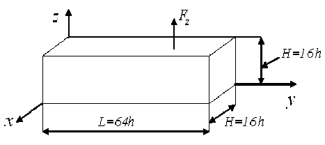
Рис. 4. Размеры КТ V ₀ ¹

Fig. 4. Sizes of CB V ₀ ¹

h = 0,5; E c = 1, where E c , E_v ( v c , v _v ) - Young's moduli (Poisson's ratios), respectively, of the binder material and fiber; at the points of the V ₀ ¹ body with the coordinates x_i , y_j , z , where z = 16 h , x i = 8 h ( i - 1), i = 1,2,3, y j- = 8 hj , j = 1,...,8 , there is a load F_z = 0,35 (Fig. 4).

The section of the V01 body in the Oxz plane is shown in Fig. 5, the fiber sections are shaded. The BM R0 CB V01 consists of single grid finite elements (1gFE) Vjh of the first order of the shape of a cube with the h side (in which three-dimensional SSS is implemented [16]). The BM R0 takes into account the inhomogeneous structure of a V01 CB within the micro-approach and generates a uniform (basic) grid with the h step of the dimensions 17 x 65 x 17.

The discrete R₁ CB V ₀ ¹ model is formed by four identical standard fourth-order 2gFEs V_q ⁽²⁾ of the cube shape, built on the V q region with the dimensions 16 h x 16 h x 16 h (Fig. 6). Fig. 5 and 6 show the

2gFE Vq(2) section and its large uniform grid with the 4h step , the nodes of the large grid are marked with dots - 125 nodes. The rigidity matrix (dimensions - 375 x 375) and the vector of nodal forces

(dimensions – 375) 2gFE are determined by the procedure described in Section 1.

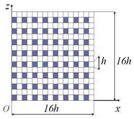
Рис. 5. Сечение КТ V ₀¹ (МнКЭ V_p ¹ )

Fig. 5. Section CB V ₀¹ (MgFE V_p ¹ )

The discrete R₂ CB V ₀ ¹ model consists of four identical small MgFEs (first type) with the dimensions 16 h x 16 h x 16 h , the sections of which are shown in Fig. 5. According to MLA, the construction of the MgFE V_p ¹ of the first type (Fig. 6) based on the standard 2gsFE, i.e., on the V_q region with the dimensions 16 h x 16 h x 16 h , is reduced to the following. In the central part of the V_q region, we select the V ₁ internal region with the dimensions 12 h x 12 h x 12 h (Fig. 7), which consists of eight identical internal 2gFEs V ₁ ⁽²⁾ of the third order with the dimensions 6 h x 6 h x 6 h (Fig. 8).

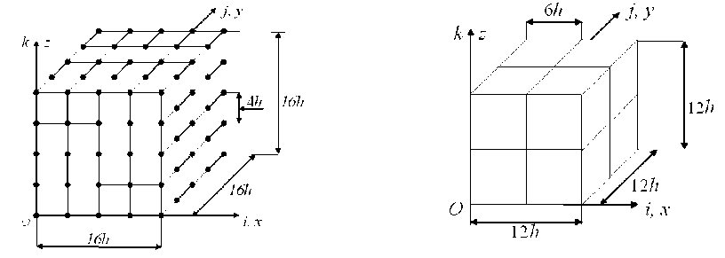
Рис. 6. Область V , 2сКЭ V ⁽²⁾ , МнКЭ V ¹ qq p

Рис. 7. Внутренняя область V ₁

Fig. 6. Region V_q , 2gFE V_q ⁽²⁾ , MgFE V_p ¹

Fig. 7. Inner region V ₁

The cross sections of the large and fine grids and the 2gFE V ₁ ⁽²⁾ are shown in figures 8 and 9. The sections of fibers (parallel to the Oy axis) of the dimensions h x h are shaded in size, the nodes of the large grid are marked with dots, 64 nodes. The rigidity matrix (dimensions192 x 192) and the vector of nodal forces (dimensions 192) 2gFE V ₁ ⁽²⁾ are found according to the procedure of Section 1. The V ₁ inner region is surrounded by eight boundary thin-walled regions V ₂ of complex shape with the dimensions 8 h x 8 h x 8 h that are identical in shape and characteristic sizes; the thickness is 2 h (Fig. 10). We build a boundary 2gFE V ₂ ⁽²⁾ on the V ₂ region using a large (uniform) grid H ₂ ⁽²⁾ with the dimensions 8 h x 8 h x 8 h with the 4 h step, i.e., of small dimensions - 3 x 3 x 3 (Fig. 11), the nodes of the H ₂ ⁽²⁾ large grid are marked with dots – 27 nodes. Fig. 10 shows a fine uniform 2gFE V ₂ ⁽²⁾ grid with the h step. Note that 8 nodes of the H ₂ ⁽²⁾ large grid lie outside the V ₂ region, but coincide with the nodes of the large grid 2gFE V ₁ ⁽²⁾ .

When constructing a 2gFE V ₂ ⁽²⁾ at all the nodes of its fine grid, the desired displacements u , v , w are expressed in terms of the nodal displacements of the H ₂ ⁽²⁾ large grid, except for those fine grid nodes that coincide with the H ₂ ⁽²⁾ grid nodes (27 nodes) and with the boundary nodes of the 2gFE

V ₁ ⁽²⁾ large grid (37 nodes), which provide docking 2gFE V ₁ ⁽²⁾ and V ₂ ⁽²⁾ . In figure 10 these 2gFE V ₁ ⁽²⁾ docking nodes are marked with dots (see Comment 3, section 1). Thus, the 2gFE V ₂ ⁽²⁾ has 64 nodes in which displacements are determined, i.e., the 2gFE V ₂ ⁽²⁾ has a rigidity matrix of the dimensions 192 × 192 and a vector of nodal forces of the dimension 192. In the V_q region, eight identical internal 2gFEs V ₁ ⁽²⁾ and eight boundary 2gFEs of the V ₂ ⁽²⁾ type form a high-precision MgFE R ¹ _p .

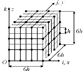
Рис. 8. Сетки внутреннего 2сКЭ V ₁ ⁽²⁾

Fig. 8. Grids of the inner 2gFE V ₁ ⁽²⁾

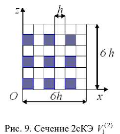
Fig. 9. Section 2gFE V ₁ ⁽²⁾

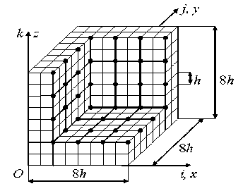
Рис. 10. Граничная область V ₂ (2сКЭ V ₂⁽²⁾ )

Fig. 10. Boundary region V ₂ (2gFE V ₂⁽²⁾ )

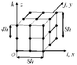
Рис. 11. Сетка H ₂⁽²⁾ 2сКЭ V ₂ ⁽²⁾

Fig. 11. Grid H ₂⁽²⁾ of the 2gFE V ₂ ⁽²⁾

Expressing the displacements of internal nodes in the MgFE R ¹ _p (using the condensation method [6]) in terms of the displacements of the boundary nodes of the MgFE R ¹ _p , we obtain a small-sized MgFE V_p ¹ of the first type. Note that the MgFE V_p ¹ of the first type has the same dimensions as the standard MgFE V_q ⁽²⁾ (Fig. 6), in which the displacement of internal nodes is excluded using the condensation method.

The results calculating CB V ₀ ¹ by MMFE using discrete models R₀ , R₁ and R₂ , are given in the table, where σ n is the maximum equivalent stress of the R n model (the σ n stress is determined according to the fourth theory of strength [33]), N_n^o and b_n^o are the dimension and width of the tape of the system of equations of the MMFE model R _n , n = 0,1, 2 . We assume that the BM CB V ₀ ¹ generates an exact solution, i.e., the σ 0 stress corresponds to the exact solution. Then the δ n (%) relative error for the σ n voltage corresponding to the R n model, where n = 1,2 , is determined by the formula

δ n (%) = 100% × | σ 0 -σ n |/ σ 0 . (8)

The analysis of the results in the table shows that the σ 2 voltage error, which corresponds to the model consisting of small-sized MgFEs V_p ¹ of the first type, is k₁ = δ ₁(%) / δ ₂ (%) = 25,122 times less than the σ 1 voltage error, corresponding to the R 1 model, consisting of standard 2gFEs V q (2) . For approximate solutions, corrected strength conditions are used, which take into account the stress error and are presented in the following theorem.

Calculation results of the models R₀ , R₁ , R₂

n	R n	σ n	δ n (%)	o n	bno
0	R 0	4,999	–	55488	924
1	R 1	4,374	12,511	1200	375
2	R 2	5,0246	0,498	1200	375

Theorem. Let the safety factor n0 of an elastic body V0 be given the strength conditions n1≤ n0≤ n2,                                                (9)

where n 1 , n 2 are given, n 1 >  1 , n 0 =σ T / σ 0 , σ T – ultimate body stress V 0 , σ 0 – the maximum equivalent stress of the V ₀ body, which corresponds to the exact solution of the problem of the theory of elasticity, built for the V ₀ body.

Let the safety factor nb of the V0 body corresponding to the approximate solution of the problem of elasticity theory satisfy the corrected strength conditions of the form nn

¹ ≤ n ≤ ² .

1 -δ α ^b 1 +δ α

Then the safety factor n ₀ of the V ₀ body corresponding to the exact solution to the problem of the theory of elasticity satisfies the specified strength conditions (9), where n b = σ T / σ b , σ b is the maximum equivalent stress of the body , corresponding to the approximate solution of the problem of the theory of elasticity, constructed for the V ₀ body and found with such an error δ _b that

| δ b | ≤δ α < C α = ^{n 2 n 1} < 1,                                 (11)

n ₁ + n ₂

where δ_α – upper estimate of the relative error δ b , δ_α is given, error δ b for the stress σ b is determined by the formula δ b = ( σ 0 -σ b )/ σ 0 , 0 < δ_α< 1.

The theorem is proved in the work [34].

It should be noted that with an increase in the δ _b error, i.e. with an increase in the δ_α estimate, the range for the n_b safety factor in the corrected strength conditions (10) decreases, becomes less than the range of specified strength conditions (9). For example, according to (11), at δ_α = C _α , the range for the corrected strength conditions degenerates to a point, which is difficult to achieve in practice. Therefore, for practice it is important to apply approximate solutions with a small error. The σ 2 stress corresponding to the R 2 model differs from the σ 0 stress of the R 0 base model (which we consider accurate) by 0,498 % (see table). For small values of the error of the maximum equivalent stresses, less than one percent, the δ_α estimate can be accepted as δ_α (%) = 1 % , i.e. δ_α = 0,01 . At δ_α = 0,01, the Δ ₁ range of corrected strength conditions (10) differs little from the Δ ₂ range of specified strength conditions (9), i.e.

A ₁ ® A 2 , where A 1 = n 2 /(1 + 8_a ) - n 1 / (1 - 8_a ), A 2 = n 2 - n 1 .

The R 2 discrete model (and the R 1 model) requires k₂ = ( N ₀ x b ₀)/( N O x b O ) = 113,94 times less computer memory, i.e., almost 114 times less than the BM R₀ CB (see Table). The analysis of the calculation results shows that the proposed small-sized MgFEs V_p ¹ ( of the first type) are more efficient than standard 2gFEs V_q ⁽²⁾ , which have the same shape, characteristic dimensions and the same inhomogeneous structure as small-sized ones.

It is important to note the following. According to Comment 2 (see Section 1), when constructing a MgFE, one can use an arbitrarily fine basic grid. Then large grids of a small-dimensional MgFE (of the first type) can have an arbitrarily high dimension and, therefore, generate local approximations of displacements of an arbitrarily high order on the internal regions of MgFE, and the number of internal regions in the MgFE increases. In this case, the order of local approximations of displacements on the boundary regions and their number does not change. It leads to an increase in the order of accuracy of low-dimensional MgFEs at a constant dimension. Nevertheless, the order of accuracy of small-sized MgFEs cannot be arbitrarily large, since the implementation of the condensation method, associated with high-order matrices, in this case requires a large amount of computer memory, which is limited.

3. Construction of small-sized MgFEs using generators of FE

The main provisions of the procedure for constructing small-sized MgFEs of the second type using generators of the FE are shown in the following example.

Example 2. We will show the main provisions for constructing small-sized MgFEs of the second type using FE generators using the example of a high-precision Lagrangian 2gFE V ₃ ⁽²⁾ with the dimensions 9 h x 10 h x 9 h (Fig. 12), where h is given, which is located in the Cartesian coordinate system Oxyz . The considered 2gFE V ₃ ⁽²⁾ is reinforced with continuous fibers with the h x h cross section that are parallel to the axis. Figure 13 shows the 2gFE V ₃ ⁽²⁾ section, the fiber sections are shaded, the distance between the fibers is h . We believe that the 2gFE bonds between the components of the inhomogeneous structure are ideal, and the displacement, stress and strain functions of these components satisfy Hooke’s law and the Cauchy relations corresponding to the three-dimensional problem of the linear theory of elasticity [16], i.e., a three-dimensional SSS is realized in the 2gFE V ₃ ⁽²⁾ region.

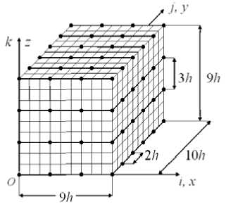
Рис. 12. Сетки 2сКЭ V ₃ ⁽²⁾

Fig. 12. Grids of the 2gFE V ₃ ⁽²⁾

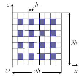
Рис. 13. Сечение 2сКЭ V ₃ ⁽²⁾

Fig. 13. Section of the 2gFE V ₃ ⁽²⁾

The 2gFE V3(2) region is represented by the BM Rd3 consisting of homogeneous 1gFE Vjh of the first order of the form of a cube with the h side [6; 7], in which three-dimensional SSS is imple- mented [16]. Figure 12 shows the basic partition Rd3 of 2gFEV3(2) , which takes into account the inhomogeneous structure of 2gFE V3(2) and generates a fine (basic) nodal uniform grid hd3 of the dimension 10×11×10 with the h step.

On the h_d ³ fine grid, we define a large uniform grid H_d ³ of the dimensions 4 × 6 × 4 with the 3 h step along the Ox , Oz axes, and with the 2 h step along the Oy axis. In figure 12 nodes of the H_d ³ large grid are marked with dots - 96 nodes. In this case, using the Lagrange polynomials [6] on the H_d ³ large grid, we represent the approximating functions u ₂, v ₂, w ₂ for the displacements u , v , w of the 2gFE V ₃ ⁽²⁾ in the following form

464       464       464

u 2 = ∑∑∑ N ijk u ijk , v 2 = ∑∑∑ N ijk v ijk ,   w 2 = ∑∑∑ N ijk w ijk ,           (12)

i = 1 j = 1 k = 1                           i = 1 j = 1 k = 1                            i = 1 j = 1 k = 1

where u_ijk , v_ijk , w_ijk – desired values of the functions u ₂, v ₂, w ₂ in the node i , j , k of the large H_d ³ grid; i , j , k – integer coordinates of the coordinate system ijk , which is introduced for the nodes of the H_d ³ large grid (Fig. 12); N_ijk – basis function of the node i , j , k of the H_d ³ grid, i , k = 1,..., 4 , j = 1,...,6, where

N ijk = L i ( x ) L j ( y ) L k ( z ),                                        (13)

where L i ( x ) = ∏ ^{4    x - x α} , L j ( y ) =   ∏ ^{6    y - y α} , L k ( z ) =   ∏ ^{4    z - z α} ; x i , y j , z k – coordinates

α=1,α≠i xi -xα            α=1,α≠jyj -yα            α=1,α≠k zk -zα of the node i, j, k of the Hd3 large grid in the Oxyz coordinate system.

Let us introduce the notation:  Nβ = Nijk , uβ = uijk , vβ = vijk ,wβ = wijk,  where  i,k= 1,..., 4 , j = 1,...,6, i.e., we have β=1,...,96. Then the expressions (12) take the form u2 = ∑Nβuβ, β=1

96 v ₂ = ∑ N _β v _β , β= 1

w ₂ = ∑ N _β w _β .

β= 1

Using (12)–(14), according to the procedure of Section 1 for 2gFE V ₃ ⁽²⁾ , we determine the rigidity matrix (of the dimensions 288 × 288 ) and the vector of nodal forces (of the dimension 288), i.e., the dimension of 2gFE V ₃ ⁽²⁾ is equal to 288 . To reduce the dimension of 2gFE V ₃ ⁽²⁾ , we use the condensation method [6]. We express the displacements of the internal nodes of the H_d ³ large grid in terms of the displacements of the H_d ³ grid nodes that lie on the 2gFE V ₃ ⁽²⁾ boundary. As a result, we obtain a 2gFE V ₃ ⁽²⁾ , which has 240 nodal unknowns. So, the dimension of 2gFE V ₃ ⁽²⁾ is 240 . Note that 2gFE V ₃ ⁽²⁾ is highly accurate, since it has the third order of approximation of displacements along the axes Ox , Oz , and the fifth order - along the Oy axis.

Let us briefly consider the procedure for constructing a small-sized 2gFE V ₄ ⁽²⁾ of the second type based on a high-precision standard Lagrangian 2gFE V ₃ ⁽²⁾ (Fig. 12), i.e., a high order of accuracy, using a generatrix of FE V_L with the dimensions 9 h × 9 h . Fig. 14 shows a fine grid corresponding to 2gFE V ₃ ⁽²⁾ and a FE V_L grid whose nodes are marked with dots – 12 nodes.

According to the FE generatrix method [21], the 2gFE V ₄ ⁽²⁾ region is obtained by parallel displacement of the generatrix of a square FE V_L along the Oy axis by a given distance d = 10 h (Fig.

15). The grid of the generating FE V_L forms a large H_d ⁴ grid of 2gFE V ₄ ⁽²⁾ . Note that the inhomogeneous structures of 2gFE V ₃ ⁽²⁾ and V ₄ ⁽²⁾ are the same. Therefore, BM R_d ⁴ 2gFE V ₄ ⁽²⁾ , like BM 2gFE V ₃ ⁽²⁾ , consists of homogeneous 1gFE V_j^h of the first order of the shape of a cube with the h side, where j = 1,..., M , where M is the total number of 1gFE V j , M = 810. BM R d takes into account the inhomogeneous structure and complex shape of 2gFE V ₄ ⁽²⁾ and generates the h_d ⁴ fine grid.

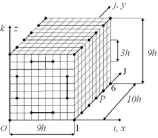
Рис. 15. Сетки 2сКЭ V ₄ ⁽²⁾

Fig. 15. Grids of the 2gFE V ₄ ⁽²⁾

9h ______J

Рис. 14. Сетки образующего КЭ V_L

Fig. 14. Grids of the generating FE V_L

According to the FE generator method, the total number N_d of nodes of the H_d ⁴ large grid of 2gFE V^ , which is embedded in the h d fine grid, is determined by the formula N_d = n xz n y , where n xz is the number of nodes of the generating FE V L , for which n xz = 12 , n y is a number of H^A 4 large grid nodes lying on the Oy axis (on the j axis), 2gFE V ₄ ⁽²⁾ has 6 nodes on the Oy axis, i.e., n y = 6 , then N d = 12 x 6 = 72 . The H^A 4 large grid nodes are evenly spaced along the Oy axis with the 2 h step. In Fig. 15 the H_d ⁴ grid nodes are marked with dots – 72 nodes. For 2gFE V ₄ ⁽²⁾ , two local coordinate systems are introduced: Cartesian Oxyz and for the H_d ⁴ large grid nodes - integer ijk , where i , j , k = 1,...,6 (Fig. 14, 15). In the 1gFE V j region, the SSS is described by the equations of the threedimensional problem of the linear theory of elasticity [16]. Consequently, a three-dimensional SSS is realized in the 2gFE V ₄ ⁽²⁾ region.

Since the grid of the generating FE V_L has 12 nodes (built on a fine grid 2gFE V ₃ ⁽²⁾ , i.e., on a fine grid of the generating FE V_L ), which in Fig. 14 are marked with dots, then to describe the displacements in the generatrix of the FE V_L , we use a third order polynomial P ( x , z ) , which in the local Cartesian coordinate system Oxz (Fig. 14) has the form [6]:

P ( x , z ) = a 1 + a ₂ x + a 3 z + a ₄ xz + a 5 x ² + a ₆ z ² + a ₇ x ² z + a ₈ xz ² +

+ a 9 xz ³ + a ₁₀ x ³ z + a 11 x ³ + a ₁₂ z 3 ,                                 (15)

where a i - constant, i = 1,...,12.

The basis function N_ijk for the i , j , k node of the H_d ⁴ large grid according to the FE generator method [20; 21] is defined as

N jk ( x , У , z ) = N k ( x , z ) L j ( У ),                                (16)

where N_ik – basis function of the node i , k forming FE V_L , corresponding to the polynomial P ( x , z ) of the type (15), i , k = 1,...,6, L j ( y ) - fifth order Lagrange polynomial:

L( У ) = fl y y ,                                (17)

p=1, p * jyj- Ур where yp -coordinate of the рth HAd grid node lying on the axis J, j //J; p, j = 1,...,6, J = 1,6 (Fig. 15).

Using (15) – (17), on the large H_d ⁴ grid approximating functions u ₂, v ₂, w ₂ for the displacements u , v , w of 2gFE V ₄ ⁽²⁾ we represent

666       666        666

u 2 =Ш N k , v 2 =Ш N^ jk , W 2 = ZZZ NW ,      (18)

i = 1 j = 1 k = 1                        i = 1 j = 1 k = 1                         i = 1 j = 1 k = 1

where u_ijk , v_ijk , w_ijk – desired values of the functions u ₂, v ₂, w ₂ in the node i , j , k of the H_d ⁴ large grid; i , j , k – integer coordinates of the coordinate system ijk , which is introduced for the nodes of the H^A_d large grid (Fig. 15); N ij _k - basis function of the node i , j , k of the H^A_d grid, i , k , j = 1,...,6.

Let us note N p = N_ijk , u в = u_ijk , v^, = v_ijk , w _p = wj_k , where u_ijk , v_ijk , w_ijk as desired displacements in the node i , j , k of the H^A_d grid; i , k = 1,6; i = 3,4, k = 2,5; i = 2,5, k = 3,4; j = 1,...,6, Fig. 14, 15, i. e., в = 1,...,72 . Then the displacement functions (18) for the H^A_d grid take the form

72                   7272

U2 =z Nвuв , v2 =Z Nвve , W2 =Z Nв we ,(19)

в=1                 в=1

where N в , u в , v e , W e — basis function of the displacements of the в ^th node of the H d grid, в = 1,72.

Using (15)–(19), according to the procedure of Section 1 for 2gFE V4(2) , we determine the rigidity matrix (dimensions 216x216) and the vector of nodal forces (of the dimension 216). To reduce the dimension of the 2gFEgV4(2) , we use the condensation method [6], i.e., we express the displacements of the internal nodes of the Hd4 large grid in terms of the displacements of the Hd4 grid nodes, which lie on the boundary of the 2gFEgV4(2) . As a result, we obtain a 2gFE V4(2) (second type) with 120 nodal unknowns. Thus, the dimension of 2gFE V4(2) is120 . By virtue of (15)–(17), 2gFE V4(2) has the third order of approximation of displacements along the axes , and the 5th order - along the axes Ox , Oz and the fifth order along the Oy axis, i.e., it is highly accurate. Note that 2gFE V4(2) has the same order of approximation of displacements along the axes Ox , Oy , Oz, the same dimensions 9h x 10h x 9h and inhomogeneous structure as the standard 2gFE V3(2) , but the dimension of 2gFE V4(2) , equal to 120, is 2 times less than the dimension of 2gFE V3(2) , whose dimension is 240. Thus, the small-sized 2gFE V4(2) of the second type generate discrete CB models of smaller dimension than the standard 2gFE V3(2) . The following should be noted. If the large and fine grids of a standard high-precision Lagrangian MgFE have a large dimension, then when constructing approximating displacement functions for the generating FE, it is advisable to use local approximations of displacements built on its fine grid. The features of the small-sized MgFEs of the first and second types are as follows. Small-sized MgFEs of the first type have a higher order of accuracy than standard ones, which makes it possible to design small-dimensional discrete CB models that generate stresses with a small error. The small-sized MgFEs of the second type have the same order of accuracy as standard high-precision MgFEs, but form discrete models of a smaller dimension than standard ones.

Conclusion

In this paper, we propose the method of local approximations (MLA) for constructing high-precision low-dimensional MgFEs, which are designed on the basis of known (standard) MgFEs. Two types of small-size MgFEs are considered. The construction of the small-sized MgFE of the first type is carried out using local approximations of displacements determined on the subdomains of the MgFE, of the second type – with the use of the generators of finite elements. The calculations of composite bodies (CB) show that the small-sized MgFE of the first type generate maximum equivalent stresses, the errors of which are 25–50 times less than the errors of similar stresses obtained using standard MgFEs, which have the same dimensions, shapes, sizes and inhomogeneous structures as being small-sized. The smallsized MgFEs of the first type for large discrete CB models generate maximum equivalent stresses with a small error. The small-sized MgFEs of the second type form discrete CB models of a smaller dimension than standard ones.