Controlling and Synchronizing of Fractional-Order Chaotic Systems via Simple and Optimal Fractional-Order Feedback Controller

Published Online June 2016 in MECS

Modeling and control topics using the concept of fractional-order of integral and derivative operators have been lately attracting more attentions, because the advancements in computation power allow simulation and implementation of such systems with adequate precision. These new concepts are aimed to improve the performance required in modeling and control of nonlinear dynamical systems. [1].

The Fractional-order Chaotic Systems (FoCS), as a generalization of integer-order chaotic systems, is a new alternative, where significant attention has been focused on developing techniques for modeling, synchronizing and controlling this class of dynamical systems. Consequently, many researchers have made large number of contributions varied from the conventional, advanced to the intelligent control approaches [2-5]. For example, A survey of fractional dynamical systems, modeling, stability analysis and control has been presented in [2]. Zhu et al. [3] presented an algorithm for numerical solution of fractional-order differential equation. Also, the synchronization of fractional-order Chua oscillator is discussed. In [4], a web- based interface is designed for fractional composition of five different chaotic systems. The interface takes initial and fractional differentiation values and yields output signals and phase portraits.

A view of the works carried out in the field of control and synchronization of FoCS, the elaboration of control law, the discretization process of fractional operators D_t ^± α , α ∈ R (resp. s ± α ), and the stability analysis are the most fundamental and important issues. It can be seen that among the most developed control and synchronization algorithms, the linear state-feedback approach in its ordinary or fractional-order form, is especially attractive and has been commonly applied due to its simplicity in analysis and implementation.

In [6], the problem of controlling unstable equilibrium points and periodic orbits is investigated via the fractional feedback of measured states. In [7], the control and synchronization of the fractional-order Lorenz chaotic system have been addressed via the fractional-order derivative approach. The single state fractional-order controller for chaos synchronization process based on the Lyapunov stability theory is presented in [8]. In [9], the fractional operators are introduced to develop a general form for synchronizing the FoCS. The authors, also, adopted the CRONE-Oustaloup method to simulate the fractional-order operators. Fractional-order PI controller for locally stabilize unstable equilibrium points of a class of chaotic fractional order systems is proposed by M. S.

Tavazoei et al. [10]. The prediction-based control technique in its fractional-form may be seen as an alternative whose objective is to enhance the desired performance [11, 12].

The stability of the nonlinear FoCS is, generally, proven theoretically by using the stability theory of fractional-order linear differential equation after linearization of nonlinear model of FoCS around the equilibrium points, or by using the Gronwall-Bellman lemma as examined in [2, 13], where the pole placement technique is derived for designing the linear state feedback controller for stabilizing a class of FoCS. In [14-16], some sufficient conditions on the stability and stabilization of a class of FoCS are proposed by using the Mittag-Leffler, Laplace transform and the generalized Gronwall inequality.

This paper uses the fractional-order control technique, addressed in [17-20], for the elaboration of a general method assigned to control and synchronize the FoCS. During the synthesis of the proposed approach, the required performances are articulated around various contradictory specifications

• ■    Simple and optimal analytical structure and parameters of fractional-order controller;

• ■    Reduced storage space memory and time execution;

• ■    Accuracy and efficiency ;

• ■    The guarantee of the stability requirements by using the sufficient conditions for the asymptotic stability and stabilization of FoCS proposed in [13-15].

The design constraints of fractional-order control approach become a dimensioning problem of analytic structure and optimization of its parameters. The discretization and learning processes analyze the tradeoff between complexities, accuracy and stability of the closed loop control system. Numerical simulations have been carried out to verify the effectiveness of the newly designed scheme by taking the fractional-order Chua’s chaotic system as an illustrative example.

The remaining part of this paper is organized as follows. Section 2 provides fundamentals of fractional calculus and its properties. Based on fractional approach, a new alternative of fractional controller to stabilize and synchronize a class of commensurate and incommensurate FoCS is proposed in section 3. The design and optimization processes of the proposed approach are detailed in section 4. Numerical simulations are presented in section 5 to confirm the validity of the analytical results. Finally, conclusion is given in section 6.

• II. P reliminaries on fractional calculus : M athematics background

Fractional calculus is a generalization of integration and differentiation to non-integer order fundamental operator cD ^ . The generalized differ-integrator may be

put forward as [21]

cD ^ f ( t ) = U,           a = 0

_x —a

J c f ( t ) d T   , a <  0

where a eR⁺ represents the real-order of the differ-integral, t is the parameter for which the differ-integral is taken and c is the lower limit, often assumed to be zero. The differentiation is then denoted D^ f ( t ) . Several alternative definitions of the fractional-order integrals and derivatives exist [1]. The three most common known definitions of fractional derivatives-integrals are Grünwald-Letnikov (GL) definition, Riemann-Liouville definition and Caputo definition. In general, the GL definition is the most suitable method for the realization of discrete control algorithms, given in time-domain as follows

GLD ^ f ( t ) = lim h ^—a • X ( — 1 )' • Г I- f ( t — i ■ h ) h ^ 0      i = 0       к ¹ J

where N = [ ( t — c )/ h ] is the upper limit of the computational universe and [•] means the integer part. h

is

the     step     time     increment     and

= (—1) •     ,  (i = 0,1,2,- ••) represents the binomial к' J

coefficients calculated according to the relation

c a c0

= a

= 1,

a a ci—1,

As shown by GL definition, the fractional-order derivatives are global operators having a memory of all past events. This property is used to model hereditary and memory effects in most materials and systems [22].

For the memory term expressed by a sum in Eq. (2), a ‘short memory’ principle introduced by Podlubny et al. [19] can be used. According to this principle, the length of system memory can be substantially reduced in the numerical algorithm to get reliable results. Some authors propose other ideas to improve the capacity of storage and computation time of fractional-order systems [23-25].

The fractional-order derivative and integral can also be defined in the transformation domain such as the Laplace transform L { f ( t ) } = F ( s ) of a fractional derivative of a signal f ( t ) , given by

L { D ±“ f ( t ) } = s ±^a - L { f^t^ -

F^

f s^k {0 D ±“ " ^{k - 1} f ( t )

k = 1     L         ¹ t = о J

Initialization function

Considering null initial conditions, the last expression is reduced to the suitable form

L { D ± ^a f ( t ) } = s ± ^a - F ( s )            (5)

The Laplace transform reveals to be a valuable tool for the analysis and design of fractional-order control systems for reasons of analysis and synthesis simplicity [22]. There are many approaches to construct and design such fractional-order controller which can be regarded as analytical 'mathematical' and learning problems of a desired performance of the controlled systems. Next, the study is concentrated around the representation models, the control modes and the stability analysis of FoCS.

• III.    S imulation , C ontrol and S ynchronization of F O CS

In this section, we mainly consider the fractional-order based feedback approach to stabilize and synchronize a large class of FoCS (identical or non identical, commensurate or incommensurate). Next, we will recall some basic definitions, remarks and theorem of the fractional-order chaotic systems [18, 25].

• A.    Preliminaries on FoCS

The most used representation of generalized form of nonlinear     fractional-order     chaotic      systems

(commensurate or incommensurate) with the control input vector u ( t ) e R ^{n x 1} is given by

F ( ^{x (} t ) )             u ( t )

Dqx ( t ) = A - x ( t ) + F ( x ( t ) ) + B - ^ ( x ( t ) )       ⁽⁶⁾

y ( t )      = C - x ( t )

where q = (qi, •••, qn)T for 0 < q < 1 is the differentiationorder vector and n is the inner dimension of the system. x (t) e Rnx1 represents the state vector with the initial condition x (t )|  ^ = x0 and A e Rnxn characterizes the constant     parameter     matrix.     The     matrix

B = diag ( sm i, --s swn ) eR ^{n x} n , where swi = 1~ n = { 0,1 } is used to designate the state variables to be controlled. F ( x ( t ) ) i—> [ 0, ro ) x R ⁿ ^ R ⁿ is a continous nonlinear function which guarantees f ( 0 ) = 0 ; moreover, f ( x ( t ) )

holds the Lipschitz condition with respect to x ( t ) , i.e., ^lim x ^ 0 I F ^{( x (} t Wl x ⁽ t )ll   ^{>0 [13]}.

Remarks.

• ■    If ( q 1 ^ q 2 ^ • • • ^ qn ) e R, system (6) modelizes the incommensurate FoCS.

• ■    If ( q 1 = q 2 =••• = qn = q ) eR , system (6) modelizes the commensurate FoCS.

• ■    If ( q 1 = q 2 = • • • = qn = 1 ) , system (6) is the

conventional representation of the chaotic systems.

• ■    The effective dimension of the system (6) is

measured by the sum of all involved derivatives Z n = 1 qi .

• ■    When u ( x ( t ) ) = 0 , there exists an unstable behavior, even chaos. In addition, the minimum value of q which results the chaotic behaviour of system      (6)       is       calculated       as

qmin = max {2 - |arg (eig (A ))| /п}       ,        where arg (eig (A))  denotes the argument of the eigenvalue of the matrix A [26].

For a given reference signal r ( t ) , which can be a constant (set point) or a function (target trajectory), the problem is to design a controller in the state-feedback form u ( t ) = ^ ( x ( t ) ) such that the state dynamics become stable. In [13-16], some new sufficient conditions on the stability and stabilization of a class of FoCS are proposed by using the Mittag-Leffler, Laplace transform and the Gronwall and generalized Gronwall inequality.

Theorem 1. [13, 14] The autonomous system (6) (with u ( t ) = 0 ) is asymptotically stable, if

■    F (x (t))       satisfies       F (0 ) = 0       and limx^0 IF(x(t))!/Ilx(t)ll = 0 ,

• ■     |arg ( eig ( A ))| >  0.5 - п - q and

• ■    q ^-|| A || > 1 .

where is the Euclidien norm, q = max ( qi ) , ( i = 1,2,---, n ) and arg ( eig ( A ) ) denotes the argument of the eigenvalue of matrix A. This system is stable if and only if |arg ( eig ( A ))| >  0.5 - q - п and those critical eigenvalues that satisfy |arg ( eig ( A ))| = 0.5 - q - п have geometric multiplicity of one.

Proof. The three necessary and sufficient conditions of this theorem are proofed and examined with detail in references [13-16].

• B.    Numerical methods to simulate behavior of FoCS

In the literature of the fractional dynamics research field, frequency and time-domain methods have been proposed for a numerical solution of fractional-order differential equations. In time-domain, two approaches are the most used in the analysis of FoCS. The GL definition [2, 3] and the improved version of Adams-Basforth-Moulton algorithm based on predictor-corrector scheme [2, 27]. Based on GL approach (2), general numerical solution of the controlled FoCS with left side derivative in the form [3]

D^x (t ) = F ( x (t)) + B • u (t) (7) can be expressed for discrete-time (tn = n • h) in the following form x (tn ) = %q • F (x (tn ))-

E C i • x ( tn - i ) + q^ • B • u ( tn ) i = 1

Ci = ^diag I cl

is a diagonal binomial

matrix, where the j-th coefficient c^qi is computed from Eq. (3) and q^ = diag ( h^q1, •, h^qn ) is a diagonal sampling time matrix. Eq. (8) is an implicit nonlinear algebraic equation respect to x ( t_n ) = ( x 1 ( t_n ) x 2 ( t_n ) •• ^T . From (8), we can construct an iterative algorithm to solve { x 1 ( t_n ) , x 2 ( t_n ), • • } , as follows

x(tn ) = qq ^ф(x(tn),x(tn-1))- n

X C i • x ( tn - i ) ^{+ q4} • B • u ( tn - 1 ) i = 1

where,

^ф(0 =

"     F 1 ( ^x 1 ( tn -1 ) v, xn ( tn -1 ) )

^F 2 ( x 1 ( tn ) , x 2 ( tn -1 ) , • • •, xn ( tn -1 ) )

_v ^Fn ( ^x 1 ⁽ tn ) ,"", ^xn -1 ⁽ tn ) , ^xn ⁽ tn -1 ) )_v

Expressions (9) and (10) are used to simulate the behavior of the FoCS, with the initial conditions x ( 0 ) = x o . The problem is to design a controller in the state-feedback form u ( t ) such that the state dynamics become stable.

• C.    Elaboration of a general method for controlling FoCS

The design approach consists of two main steps similar as in [28]. The first one is to eliminate the nonlinearity in (6) and the second one is to make the system dynamics asymptotically stable.

This strategy can be seen as a distributed fractional control approach which preserves the topology and flexibility of decentralized control yet offers a nominal closed-loop stability guarantee. In order to eliminate the nonlinearity term F ( x ( t ) ) in (6), we define the control signal as follows

u (t ) = ^( x (t))-F ( x ( t )) (11)

The linear part ф ( x ( t ) ) acts as an external input to stabilize the system dynamics. Figure 1 summarizes the block diagram of the developed control approach of the FoCS.

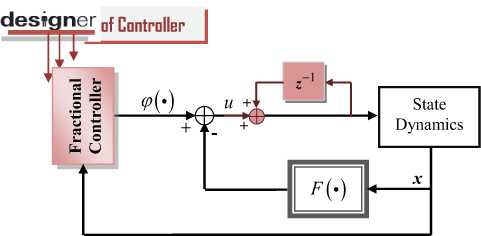
Fig.1. Block Diagram of the Developed Control Scheme.

To cancel small oscillations, if they persist, the addition of an integrator, as illustrated in Figure 1, can be seen as an appropriate solution. The control function ^ (•) is defined in its generalized form as

ф ( x ( t ) ) = u ( t ) = - G • Dqx ( t )          (12)

If q = 0 , the model (6) is just the state feedback control law. If q e [ 0,1 ] , the system dynamics (6) become

Dtqx ( t ) = A • x ( t )                 (14)

where A = ( I + G • Sw)   • A , I is the identity matrix, and G is the feedback gains to be determined. Therefore, our aim is to design a suitable feedback matrix gains G such that the system dynamics (14) is asymptotically stable.

Theorem 2. If feedback matrix gains G is chosen such that

■     F ( x ( t ) ) satisfies lim x ^0 | A ( x ( t ))||/|| x ( t )|| = ⁰ ,

■

a arg ( eig ( A

> 0.5 - n - q and

■

q -I A ll >¹ .

Then, the controlled system (14) is asymptotically stable.

• D.    Elaboration of a simplified form of FoC algorithm

In order to reduce the amount of historical data (‘the growing calculation tail’ and finite microprocessor memory [19, 29]), improve the accuracy of the numerical solution and derive the recursive control algorithm, a Simplified and Optimal analytical Form ‘structure and parameters’ of the Fractional-order Feedback (SOF-FoF) model of the fractional-order controller (12) is proposed. The fractional feedback state control (12) is defined in its incremental form by using the GL definition given by Eq. (2), as

ф ⁽ x ⁽ tn ) ) = u ⁽ tn ) = G ‘^ qx ⁽ tn )

= - G -

n

* - Co - x ( tn ) +h- ^ C j -

.                    j = 1

^x ( tn - j )

size_net

- ^-   ^ ^u PI Reg; ⁽ tn )

i = 0       _   ⁶¹

where, uPI_Regi

( tn ) = [ K2i  K2i + 1 ]'

^x ( tn - 2 i )

^x ( tn - ( 2i + 1 ) )

and

Ki = ( G -й) - C i , ( i = 0,1,2,-,size_net ) ,

Cj = diagfcq1,cq2,---,cqn ) and Cq=InXn j       ^ j j       J )                  (17)

Й = diag ( h q ¹, h ^{q 2},---, h qⁿ ) ,

G = diag ( ^g1,^g 2^,■•■^{, g}n )

where gi , i = 1,2< • •, n is the elementary i-th control gain and 0^ is computed from Eq. (3).

Based on the mathematical formula of the ordinary PI controller outputs, expression (15) can be seen as an infinite sequence of linear regulators modeled by an infinite distributed network of PI controllers temporarily shifted.

Each node in the network represents an elementary PI-subsystem with modified gains Ki , ( i = 0,1,2,---,size_net ) and size_net e N is the size of distributed PI-network measured by the number of additive PI-subsystems in the network. Figure 2 summarizes graphically the main idea of the formulation of the proposed i -th control law (15).

The number of nodes in the network { size_net } is the chosen function of the desired performances { Dp (•) } , such as the accuracy (measured by the precision { ^d } ), the computation steps { h } and the memory storage requirements { Lm } , as

0 <  size_net < [ D p ( h , L m , § d ) ]       (18)

where [•] is the integer part.

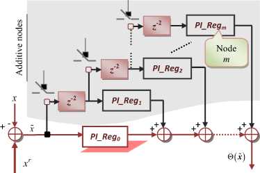
Fig.2. Equivalent Model of the SOF-Fof Approach.

It can be conclude that the analytical form (15) makes the simulation and implementation of fractional-order controllers much easier and enables a smooth transaction for real applications to take advantages of this new approach. Moreover, the effectiveness of the proposed controllers remains to be approved through application examples in different industrial and scientific disciplines.

• E.    Elaboration of a general method for synchronization of FoCS

In this section, we mainly consider the synchronization process of two identical FoCS (in form (6) and order q ). Furthermore, there are two general properties of the fractional-order calculus are used, such as

• ■    D ^ D ^ f ( t ) = D ^ D ^ f ( t ) = D f^{+ в} f ( t )

• ■    Dq ( a - f ( t ) ± p - g ( t ) ) = a - Dqf ( t ) ± Д - Dqg ( t ) 0 <  q <  1,   { a , в } е>

Consider a fractional-order system of vector orderq = (qi, ...n qn)T e[0,1], described by

<

, Dtxm = Am • xm + Fm ⁽ xm ) ^ xm ⁽ 0 ) = xm о

where xm e Rn denotes the systems’s n-dimensional state vector, Am e Rnxn is a constant matrix and Fm : nn is the nonlinear part of the system. We consider the system (19) as the drive (master) system, and then the response system (slave) is given as dSxs = A • x„ + Fs (xs) + B -0(xw,xs) ts ss ss    ms

, xs ( ⁰ ) = xs 0

where 0 ( - ) e R ⁿ is the control function. xs , F_s ( x_s ) and As imply the same roles as x_m , F_m ( x_m ) and A_m in the master system, respectively.

The chaotic synchronization between drive system (19) and response fractional order system (20) belongs to the problem of tracking control, i.e., the output signal x_s of system (20) follows the reference signal x_m ultimately. Let e = x_m - xs be the error vector of system (19) and (20). Then, subtracting system (20) from system (19), the synchronization error dynamics is designed as

^D tq ^e = Am •^{e +} [ Am  As ]• ^x s ⁺

[ ^F m ⁽ xm ) ^F s ^{( x} s ) ]  ® ^{( x} m

, x_s

)

If the control parameters of chaotic systems drive and slave are identical, i.e., A_m = As , system (21) becomes

^Dt^e = Am * ^{e +} [ ^Fm ^{( x}m ) ^Fs ^{( x}s ) ] ® ^{( x}m , ^xs ) ⁽²²⁾

It can be observed that the synchronization error system (21) (resp. (22)) contains two parts. The first is the linear part modeled by A_m • e and the nonlinear other part modeled by { [ Fm ( xm ) - F ( xs ) ] } .

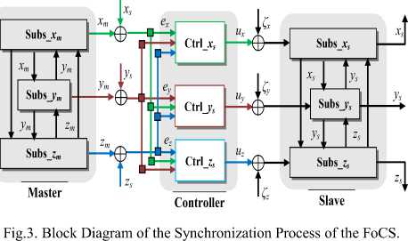
Figure 3 summarizes the block diagram of the synchronization process for the three-dimensional perturbed fractional order nonlinear systems.

Moreover, it can be observed that the controllers Ctrl_ x_s , Ctrl_ y_s and Ctrl_ z_s share information in order to improve closed-loop performance, robustness and stability. This strategy can be seen as a distributed fractional control approach which preserves the topology and flexibility of decentralized control yet offers a nominal closed-loop stability guarantee.

Our goal is to design an appropriate feedback controller 0(xm,xs) , such that the trajectory of the response system (20) with initial condition xs (0) asymptotically approaches that of the drive system (19) with initial condition xm (0) and, finally, implement synchronization, in the sense that lim ||e(t)||= lim ||xm -xs || H> 0         (23)

t M-ro          1 1-0-^

where     is the Euclidian norm. Therefore, the control function @(xm, xs) , is chosen such that the error dynamics (21) become stable.

To simplify the study, the approach consists of two main steps. The first is to eliminate the nonlinearity in (21) and the second is to make the system dynamics asymptotically stable. In order to eliminate the nonlinearity term

{^(xm, xs) = Fm(xm(t))- Fs(xs(t))+ [Am - As ] ’ xs} in (21), we define the nonlinear control law as

Next, we propose the linear control law similar than the previous section, such that

U (t ) = G • Dqe (t)

where G >  0 is the feedback matrix gains which is always diagonal. Thus the error dynamics (25) become

Dqe (t) = A • e(t)

where A = ( I - G • S^ ) • A_m , I ^{n x n} is the identity matrix and the feedback gain G e R ^{n x n} needs to be determined. The design procedure consists of spotting the matrix gains G to stabilize error dynamics (26).

Theorem 3. The error dynamics (26) is asymptotically stable, if

■

Fm ( xm )

satisfies

^lim xm —0ll ^F ( x m )ll/ll x m ll = ⁰

seen as an appropriate solution.

■

■

and Fs ( xs ) satisfies lim

Xs ——0

> 0.5 * n * q and

||^F ( x s )||/ INI = ⁰

^q *1 PA ll> 1.

where q = max ( qi ) , i = 1,2, • • • and eig ( A ) represents the

eigenvalues of matrix A .

Based on the used reasoning in the previous SOF-FoF approach (15), the general form of the linear part of the control law used in the synchronization of identical FoCS is given in its simplified form as

size_net

u ⁽ tn )= E ^u pi Reg- ⁽ tn ) i = 0     _

^u PI_Reg _i

⁽ tn ) = _ K2i  K 2 i + 1 ]*

e ( tn - 2 i )

^e ( tn - ( 2 i + 1 ) )

Ki = ( G * A • ) * C i , i = 0,1,2, • • • ,size_net

IV. M ultiobjective O ptimization of the SOF-F of C ontrol L aw

To design an optimal controller, an efficient optimisation technique should be used. In particular, the evolutionary computations has received considerable attention in recent years. In this work, Genetic Algorithms (GAs) have been proposed as a learning method that allows automatic generation of optimal structure and parameters of the fractional controllers, which can be represented as an extremum problem of optimization index. Algorithm 1 shows the schematic process of GA used in this work. The chaotic mutation operator [30] is used to solve the problem of maintaining the population diversity of GA in the learning process. The concept of elite strategy is adopted, where the best individuals in a population are regarded as elites.

where G , h and C _i are diagonal matrices given in (17). Therefore, the nonlinear control function ensures the synchronization between the systems (19) and (20) will be obtained as

®O = u(tn ) + ГFm (xm (tn )) Fs (xs (tn ))"|

⁺ [ Am ^- As | * ^xs ⁽ tn )

The linear part U ( t_n ) acts as an external input to synchronize the system master-slave as shown in Figure 4. The nonlinear part T ( x_m , x_s ) is considered to eliminate or reduce the effect of the nonlinearities F_m ( * ) and F_s ( * ) . The linear part acts as an external input to synchronize the system master-slave.

Algorithm 1. Basic structure of the used GA.

• 1.    Begin

• 2.     gen : = 0;

• 3.     Initialize ( P ( gen ));

• 4.    Evaluate ( P ( gen ));

• 5.    Keep_The_Best_Individual ();

• 6.    while (not_stopping_criteria ( P ( gen ), gen )

do

• i.    gen : = gen +1;

• ii.    Select (( P ( gen )) from ( P ( gen -1));

• iii.    Crossover ( P ( gen ));

• iv.    Mutate ( P ( gen ));

• v.    Evaluate ( P ( gen ));

• vi.    Elitism_strategy ( P ( gen ));

• 7.     end ;

• 8.     end .

The parameters to be optimized are obviously the controller gains and the number of PI-subsystems uncluded in modeling of control law (network nodes). So, the optimized parameter set may be such that

x s

des j 9ner of Controller

u

-

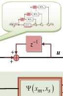
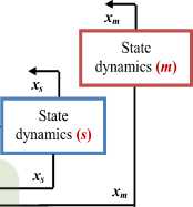
Fig.4. Block Diagram of the Developed Synchronization Approach.

Kb = |_ G ctrl   ^S net _| ,

< G ctrl =_ 8 1  - • gn ] T ,                  (29)

S net = _size_net1 • • •  size_net _n ] T

To cancel small oscillations, if they persist, the addition of an integrator, as illustrated in Figure 4, can be

The key to put a genetic search for the SOF-FoF into practice is that all design variables to be optimized (29) are encoded as a finite length string, called chromosome. To simplify the genes coding mode, i.e., avoidance of the mixed coding (real-integer) and the genetic operators adapted for each mode, the real coding is used with the restriction

^size_net m =[ ^ retpi m JeN+,

' ^ retpi m ^e

0, ^Lm h

( i = 1,2,-

n ) ;

| arg ( eig ( A ))|

П — q ■   >

_ g ² ^q -| l A I - 1 >  0

0,

0 <  gi <  g max ^{e R}

where 7 _netpi modelizes the number of nodes in the network, size_net e N+, included in modeling of SOF-FoF control law (15) and [ x ] represents the integer part of x . Every chromosome (Figure 5) which encodes the knowledge base of the SOF-FoF model can represent a solution of the problem, that is, a SOF-FoF optimal knowledge base.

Configuration factors

M_x = [ Nh ] denotes the integer number of computing steps, n is the number of state variables to be controlled and N represents the running time. size_net is a number of PI-subsystems and Max_net characterizes the upper limit of PI-subsystems in control law. The additional constraints are the lower 0 = KT and upper

T

0 = K^ limits of the parameters to be optimized. The optimization problem (31)-(32) can be transformed to an unconstrained problem via the Exterior Penalty Function (EPF) [31] given by

Controller gains

Fig.5. Chromosome Structure of the Knowledge Base of SOF-Fof Model.

n

Min G ( 9 ) = X wi "

S eR   i = 1 v

n

X JC (•)   + n ( 9 )   (33)

i        S eR

V c = 1

where П ( S ) is the EPF, expressed as S eR

In this paper, the optimization process is to find the optimal knowledge base (29) of the SOF-FoF model, while satisfying the objectives and constraints specified by the designer such as simplicity, precision (accuracy), fewer energetic effort and overall stability conditions guarantee.

The simplicity of the control law is measured by a combination of a reduced (optimal) number of PI-subsystems while keeping a prescribed level of efficiency ^ d , x ( tn ) - x ( tn - 1 )| < d in the control process and | xm ( tn ) - xs ( t_n ) < C in the synchronization process. The general optimization procedure may be pronounced as follows

Find the knowledge base K_b (29) that minimize the objectives Ji , i = 1,2,3 , such that

In

l

n (^) = rh • X(hk (Ol

•9 ^е®         L k = 1

" РГ /

g

this application, hk = 0, V k e N . The weights

( wi , rg , rh ) > 0 can therefore, be used in the control system conception as design parameters to tradeoff between different weights of performance specifications (better accuracy, a reduced consumption of energy control, optimal structure and satisfied stability analysis conditions). From (33) and (34), the local and global minima can be calculated if the region of realizability of i 9 is convex [32]. It is usually assumed that

X ( wi , rg , rh ) = ¹ i

i

J ₂

i

Mx ¹

■ X l ei ( tkнЛ k= 0^{1               1}

Ф and

1 N ,

:-1 ■ X Vit (tk )

k=0

i = 1,- --, n

The fitness function used by the GA, can then defined as

Fit ( S ) =

S eR

d + G ( 9 )

S eR

and satisfying the design constraints g , such that

where (d, 5)e R2 and 8 is a small positive constant used to avoid the numerical error in dividing by zero. The algorithm stop criterion is fixed by a maximal number of generation, or by a required precision values specified by a given error.

• V. C ontrol and S ynchronization of F ocs V ia SOF- F of A pproach

In this section, we apply the proposed design in stabilizing and synchronizing the fractional-order Chua’s oscillator to verify its effectiveness.

• A.    Description of fractional-order Chua’s oscillator

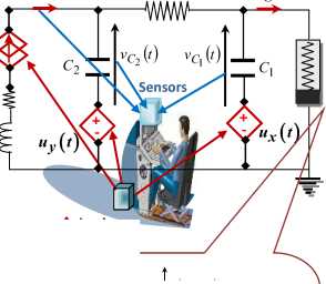
The mathematical model of the circuit can be obtained by applying the Kirchhoff’s laws into the circuit depicted in Figure 6.

ig ( t )

i L ( t )

R uz ( t )

RL

L

g

Actuators

Slope = G _b

g ⁽ C r ⁽ t ) )

Slope = G _a

Slope = G _b

Fig.6. Diagram of Chua’s Circuit under Numerical Control Computer.

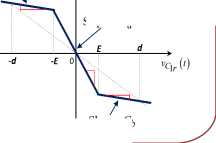
The integer-order of derivative and integral operator in classical form of Chua's circuit dv^ ( t )/ dt , dvc^ ( t )/ dt and di_L ( t )/ dt are replaced by the fractional operators d^q1 ^V C1 r ( t )/ dt^¹, dq² vc2_r ( t )/ <10 ² and d ^q 3 iLr ( t )/ dtq ³ , respectively, where q1 e Ж is the real-order of the capacitor Q_r , q 2 e Ж is the real-order of the capacitor C2_r and q g e Ж is the real-order of the inductor L_r .

By defining the rescaling xr (t ) = vC1 r (t)/E, Уг (t ) = vC2 r (t)/E, zr (t) = iLr (t)/(E • R), a = C2r/C1 r, в = C2r/(Lr • G2), m0 = Ga/G, Y = C2r • RLr /(Lr • G), G = VR,, mi = GblG we can transform the main expression of Chua’s circuit into the corresponding dimensionless form [3], with the addition of the adjustable voltage and current generators, as a generalized form where,

g ( xr ) = m1 • xr + g (xr )

= 0.5 • ( m ₀ - m 1 ) • (| x_r + 1| -1.

I xr ^- 1 )

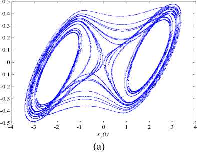
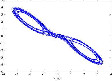
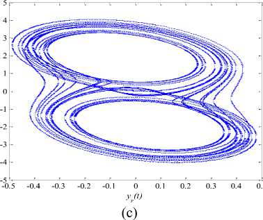
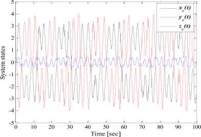
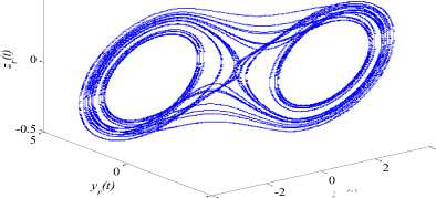
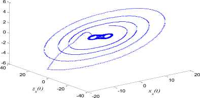
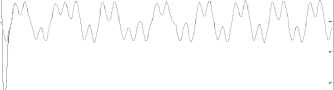
Typical values of the system parameters a = 10.725, p = 10.593, у = 0.268, m 0 = - 1.1726 and m i = - 0.7872 create chaotic behaviour ‘chaotic attractor’ in the dynamical systems (37) as indicated in Figures 7 (a)-(e). We have selected the initial conditions as ( x_r ( 0 ) , y_r ( 0 ) , z_r ( 0 ) ) = ( 0.2, -0.1, 0.1 ) and the derivative orders are chosen to be ( q_x , qy , q_z ) = ( 0.93,0.99,0.92 ) [2]. The calculus step is chosen as h = 0.01 [ sec ] for numerical simulations.

(b)

(d)

(e)

Fig.7. Phase Planes and Time Responses for The Uncontrolled Fractional-Order Chua’s Oscillator.

-5   -4

xr(t)

The first case corresponds to the control of the fractional-order Chua’s oscillator (37) at the origin. Here, the contribution is illustrated in the fractional chaos control context.

The second case corresponds to the synchronization of two identical fractional-order Chua oscillators. Here, the contribution is illustrated in the fractional chaos synchronization context.

• B.    Control of fractional-order Chua’s oscillator via SOF-FoF approach

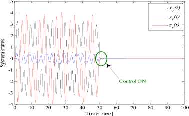
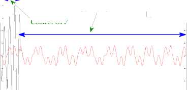
In this application, the reference model is chosen to be xr = [ 0 0 0 ] ⁷ at time t = 50 [ sec ] , i.e ., the SOF-FoF controller was applied at time t = 50 [ sec ] to stabilize the state x ( t ) of the fractional-order Chua’s oscillator at the equilibrium point (origin).

Table 1. Specifications of the GA learning.

Characteristic	Value
Population Size	20
Number of max generation	1000
Coding chromosome	Real
Gain factors gi - ( i = 1,2,3 )	[10-4, 1.0]
Number of regulators ^ netpi i { i=1,2,3 }	[0.0, 1/0.01]
Selection process	Tournament
Arithmetic Crossover	P c = 0.6
Chaotic Mutation	P m = 0.08

The MGA characteristics are summarized in Table 1, with the chromosome structure schematized in figure 8. The knowledge base to be optimized (37) has the dimension of three, i.e , n = 3.

Around 200 optimization iteration steps (generation number), the knowledge base of the SOF-FoF model is obtained as

KbT

{ 0.8976, reg₀ + 1 } { 0.4184, reg₀ + 0 } { o.92O5, reg0 + 1 }

Stability analysis: The knowledge base (39) is chosen in order to guarantee the asymptotic stability of the system dynamics (14), i.e ., satisfy the three conditions of Theorem 2.

• ■    By applying the inequality \a + ( — b )| < | a | + |— b |, it is easy to verify that F ( x ) = —a* g ( x ) satisfies F ( x ( 0 ) ) = 0 and

  lim x > 0

  
  

  II ^{F (} x ⁽ t ))ll

  
  

  II x ⁽ t )ll

  
  

  lim

  x ^ 0

  
  

  < lim

  x ^ 0

  
  

  xr +

  
  

2   2

+ yr + zr

•( mo — m1 )-(|xr| +1 — I xr|— 1 ))2

2   2

+ yr + zr which implies that F (x (t)) satisfies condition 1 of Theorem 2.

• ■    For the system matrix of (17), we get the eigenvalues        ^ 1,2 =— 0.1021 ± 1.8682 • j       ,

  X3 = — 6.2942. All eigenvalues satisfy condition 2 of         Theorem         2,         where

  I arg ( 4 1,2 )| = 1.6254 >  0.99 • 0.5 • n = 1.5551          and

  |arg ( 2 3 )| = n >  1.5551.

• ■    According to the condition 3 of Theorem 2, where q J| л || = 0.99 -11.3038 = 12.8772 > 1  , the

system is asymptotically stable.

Figure 8 (a) shows the evolution of the system states. It can be remarked that the states of the Chua’s circuit have been regulated effectively and efficiency to the equilibrium point ( x^ , y^Tr , z^rr ) = ( 0, 0, 0 ) and the control objective is attained. From Figure 8 (a), in point of reference signal transitions, we can observe that the effect of coupling between the three controlled variables was reduced. This is a good compensation of the interactions between the state variables. The controller was able to ensure convergence with relatively short transient responses. The corresponding input signals of the system are depicted by Figure 8 (b). Simulation results displayed in Figures 5 (a)-(c), show that the zero solution ( 0, 0, 0 ) T of the controlled fractional-order Chua’s oscillator is globally asymptotically stable.

(a)

ux(t) uy(t) u (t)

-1

0     10    20    30    40    50    60    70    80    90    100

Time [sec]

(b)

Fig.8. Stabilization of Fractional-Order Chua’s Oscillator at the Origin using SOF-Fof Approach: (a) System States. (b) Linear Control Signals.

It is noted that the SOF-FoF approach provides slightly faster responses to set-point changes, with only small overshoots. The decoupling capabilities resulting from the design technique were generally good.

• C. Synchronization of fractional-order Chua’s oscillator via SOF-FoF approach

In order to observe the synchronization behavior in two identical fractional order Chua systems, we construct a master-salve configuration with a master system given by the fractional-order Chua’s oscillator comprising three state variables denoted by the script m (abbreviation of master) and with a similar chaotic system with three state variables denoted by the script s (abbreviation of slave). The drive (master) and the response (slave) are described by the following differential equations.

• ■    The drive system is described by

Dt x ^xm = ^{a - ( y}m  ^xm  g ^{( x}m ) )

q y                                  (41)

Dt ym = ^xm ym + zm

Dt z ^zm = ^- P ^- ym ^{- у - z}m

• ■    The response system is given by

Dt x xs = a • ( ys ^{- x}s ^- g ( ^xs ) ) + swx • ux

• -    Dt Уз = xs ^- Уз + zs + ^swy ^- uy         (42)

The main objective is to design the controller u = [ux, Uy, uz J based on the developed SOF-FoF approach (27) so that the response system (42) asymptotically approaches the driving system (41), and that the limit of the synchronisation error vector e = ^ex, ey, ez J approaches zero, where ex = xm - xs , ey = ym - ys and ez = zm - zs .

In the numerical simulations, we also set the calculus step as h = 0.01 [sec] and the system parameters are as : a = 10.725, в = 10.593, у = 0.268, m0 =-1.1726 and m1 =-1.7872 and (qx,qy,qz) = (0.93,0.99,0.92) . The initial conditions of the drive system are (xm (0), ym (0), zm (0)) = (0.2, -0.1, 0.1) and the initial conditions of the response system are selected as: (xs (0), ys (0) ,zs (0)) = (3.0, 2.0, - 1.0) [3].

From Figure 9, it is evident that, when ( swx = swy = swx = 0 ) , the trajectories diverge from each other due to the sensitivity to the initial conditions. However, as soon as the controller (28) is applied, not only tracking of the reference signal but also synchronization of all the state variables is achieved. In this application, the control law is applied at time t = 10 [ sec ] .

Around 450 optimization iteration steps (generation number), the knowledge base of the SOF-FoF model is obtained as

{ 0.8624, rego + 1 } { 0.0154, reg₀ + 0 } { 0.3526, reg₀ + 2 }

For the system matrix of the system (17), we get the eigenvalues X₁₂ =- 0.1951 ± 3.9144 - j , X ₃ =- 78.9565 . All eigenvalues satisfy condition 2 of Theorem 3, where | arg ( ^ 1,2 )| = 1.6206 >  0.99 - 0.5 - n = 1.5551 and | arg ( 4 ₃ )| = n >  1.5551.

According to the condition 3 of Theorem 3, where q -||A 11 = 0.99 - 155.8866 = 154.3278 >  1 , the system is asymptotically stable. Then, the system (26) can be stabilized to the origin point, i.e., synchronization of system (41) and (42) is achieved.

From Figures 9 (a)-(d), in point of reference signal transitions, we can observe that the effect of coupling between the three controlled variables was reduced. This is a good compensation of the interactions between the state variables.

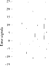
The controller was able to ensure convergence with relatively short transient responses as depicted in Figures 10 (a). The numerical results, illustrated in Figure 10 (b), shows that the error system is driven to the origin point fast, i.e., the systems (41) and (42) are synchronized.

-15

Control ON

--------zs(t)

----zm®

-5

-10

Control OFF

-20

-25

0     10    20    30    40    50    60    70    80    90    100

Time [sec]

(c)

(d)

Fig.9. The Orbits of the Three States of Drive and Response Systems: (a) Xs — Xm . (b) Уз — Ут • (c) Zs — ^zm . (d) The portrait in R"3 .

-5

-10

Control ON

-------xs(t)

---- xm^

Control OFF

-40

-20

u (t) u (t) u (t)

-60

0     10    20    30    40    50    60    70    80    90    100

Time [sec]

(a)

-20

0    10    20    30    40    50    60    70    80    90    100

Time [sec]

-20 0

ex(t) ey(t) e (t)

5          10         15         20         25         30

Time [sec]

(b)

Fig.10. Time Response of the (a) Control Inputs and (b) Synchronization Errors between Drive and Response Systems of the Fractional-Order Chua’s Oscillator.

Simulation results show the good performance of the developed algorithm and confirm the effectiveness of the control law in the tracking of the desired trajectories.

• VI. C onclusion

Progress has been made in coupling advanced modeling and controlling methods to chaotic dynamical systems. In this paper, a simple and optimal form of fractional-order feedback approach assigned for the control and synchronization of a class of FoCS is proposed.

The proposed design and optimization of SOF-FoF model represents a powerful and simple approach to provide a reasonable tradeoff between computational overhead, storage space, numerical accuracy and stability criterions in stabilization and synchronization of a class of FoCS.

The advantages of the proposed designing methodologies are that they reduce the dimension of fractional configuration, search the optimal knowledge base, minimize the storage space and computational time while maintaining almost the same level of desired performances.

Finally, due to the fact that the generated real-time executable runs on the processor of a computer and the memory constraints are not so critical. Thus, an optimal implementation of the SOF-FoF model will be possible.